• We release Krea Realtime 14B, a 14-billion parameter autoregressive video model distilled using Self-Forcing, capable of real-time, long-form generation
• Our model is over 10x larger than existing realtime video models
• We introduce novel techniques for mitigating error accumulation, including KV Cache Recomputation and KV Cache Attention Bias
• We develop memory optimizations specific to autoregressive video diffusion models that facilitate training large autoregressive models
• Our model enables real-time interactive capabilities: Users can modify prompts mid-generation, restyle videos on-the-fly, and see first frames in 1 second

Read on for a deep dive into how we scaled Self-Forcing to a 14B model and the novel inference techniques we engineered to unlock stable, long-form video generation.

To understand the techniques used to train Krea Realtime 14B, we must first examine why existing video generation models are incompatible with real-time streaming, and how converting them to autoregressive architectures introduces new problems.

Most state-of-the-art video diffusion models, like Wan 2.1 14B, use bidirectional attention. This means that all frames are denoised in parallel, and all frames in a sequence can attend to each other. This means the future frames can influence past frames, and vice versa.

In contrast, autoregressive or causal models can generate videos by fully denoising one frame—or blocks of frames—at a time.

This bidirectional attention makes the task fundamentally easier for the model: it is better able to correct its errors over the course of denoising, and the attention is more expressive. However, denoising the entire video sequence in parallel makes it impossible to stream frames back to a user in real-time.

In autoregressive models, once a frame has been fully denoised, it is immutable. Subsequent frames can attend to it, but not change it retroactively. This means that once a frame is generated, we can immediately show it to the user, enabling streaming video generation.

While this capability is attractive, training autoregressive models from scratch can be slower because it requires custom attention masks and, according to CausVid, they tend to underperform bidirectional models. Existing literature like Diffusion Forcing, Teacher Forcing, and Causvid thus seek to convert pretrained bidirectional models into causal ones rather than training autoregressive models from scratch.

This causal structure is a natural fit for real-time applications, but there is a key flaw in existing autoregressive training and distillation methods: exposure bias.

Existing works train autoregressive models by using attention masks that allow each frame to attend only to past frames. They simulate the autoregressive inference task by using real video data as context. Teacher Forcing allows the model to attend to clean latents of past frames, while Diffusion Forcing uses noised latents as context. In both cases, the context comes from ground truth frames from the training dataset.

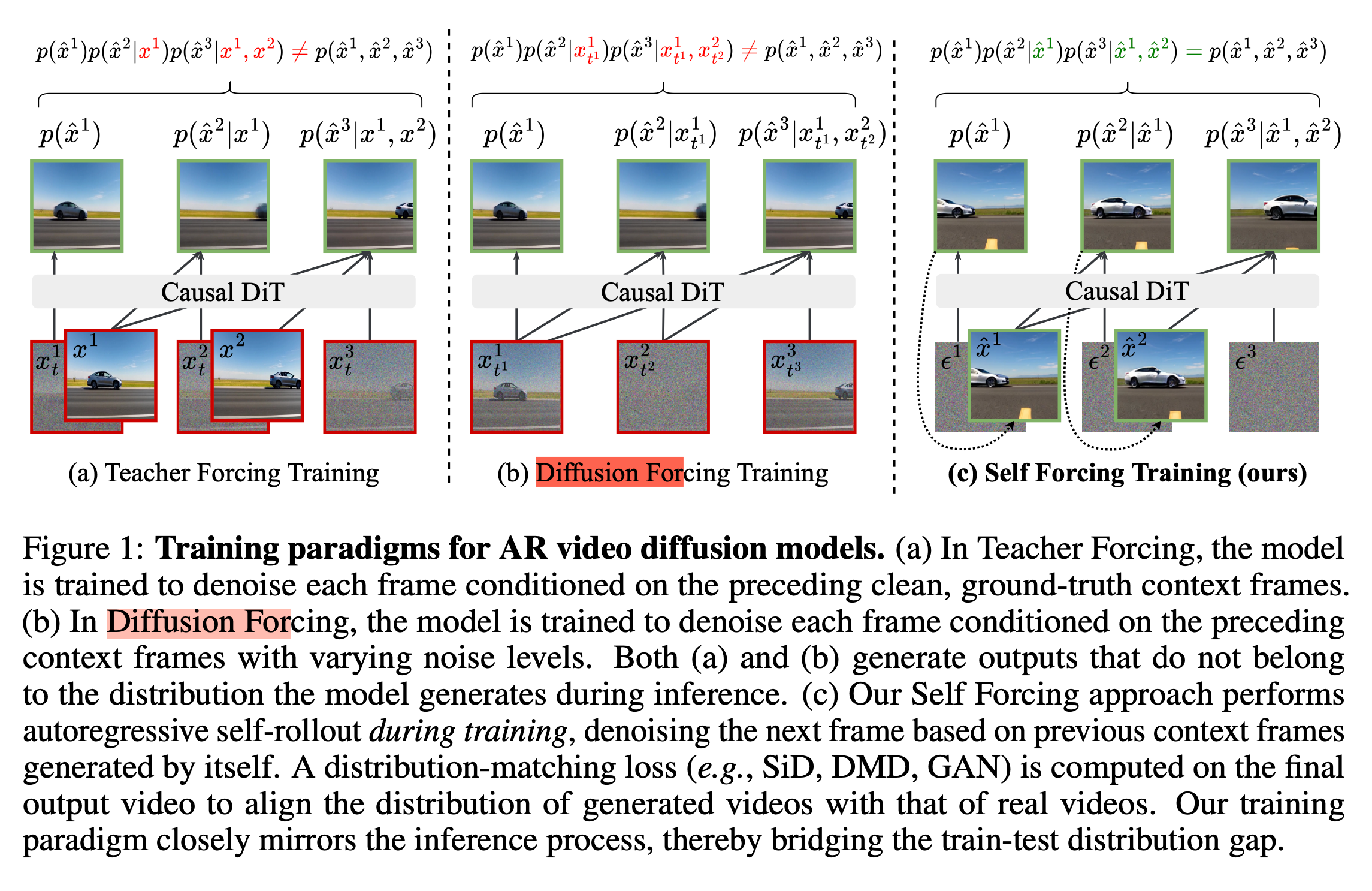
Figure 2: A comparison of different context strategies in autoregressive video models. Source: Self-Forcing

However, at inference-time, the model will be conditioned on past frames generated by itself. This is a significantly different distribution from frames in the training data, even if they are noised.

This creates a critical train-test mismatch known as exposure bias. During training, the model learns to predict the next frame given a context of (potentially noised) frames from the dataset. At inference-time, however, the model must predict the next frame using its own, imperfect previous generations as context.

Because the model is never "exposed" to its own mistakes during training, it doesn't learn how to recover from them. A minor artifact in one generated frame is fed back as input for the next, often causing a cascading failure where errors accumulate and rapidly degrade video quality.

Self-Forcing bridges this gap by performing autoregressive generation during training - the model generates each frame conditioned on its own previous outputs, exactly as during inference. This enables holistic video-level losses that evaluate entire generated sequences. It is also a data-free training pipeline, leveraging the knowledge of pretrained teacher models.

The self-forcing distillation process uses 3 stages:

1. Bidirectional Timestep Distillation

The timestep distillation maintains bidirectional attention (all frames are generated jointly), but reduces the number of sampling steps the model needs to generate a video from ~30 to 4 steps. This initial efficiency gain is a prerequisite for realtime inference, and for the Distribution Matching Distillation training stage that follows, allowing us to tractably sample from the model at train time.

2. Causal ODE Pretraining

This pretraining introduces the model to the causal generation task, providing a stabler initialization for the next stage of training.

We use prompt data to generate synthetic ODE solution trajectories from the undistilled teacher model. We then apply an attention mask which mimics the final autoregressive task to the timestep-distilled student model, and use a regression loss to match the sampling trajectory of the teacher.

Figure 3: A block-causal mask with 3 blocks and 3 frames per-block

As shown in Figure 3, the mask allows:

• All frames within a block to attend to each other
• All frames to attend to all past frames

We call this a "block-causal" mask, as attention is bidirectional within a block, but causal between blocks. Note: for notational simplicity, we use the terms "frame", "latent frame" and "latent frame block" interchangeably.

3. Self-Forcing Distribution Matching Distillation

We use the student model to autoregressively sample videos, matching the inference-time task. We then use the Distribution Matching Distillation (DMD) objective to steer the model's output distribution towards high-probability regions. The method uses two bidirectional diffusion models to estimate score functions of real and fake distributions, using their difference as a gradient to improve the generator.

A distribution-level loss is essential for us to leverage the knowledge of a bidirectional video model as a teacher. A loss that matches the internal states of student and teacher wouldn't make sense between a model with bidirectional attention and a model with causal attention.

Also, using pretrained diffusion models as score estimators allows us to train without real video data, which makes DMD an appealing choice compared to other methods that use distribution-level losses but include real data.

While the Self-Forcing paper provides a strong blueprint, scaling the technique to a 14B model—over 10x larger than the original work—introduced significant memory and engineering hurdles. This section details the novel optimizations and adaptations we implemented at each stage to make this scale-up successful.

Timestep Distillation

For this stage, we used an existing open source few-step distillation of Wan 2.1 14B by LightX2V.

Causal ODE Pretraining

For this pretraining, we adapt the code from Causvid. While the authors use a timestep shift value of 8 for their training, we find that this leads to less dynamic motion and worse high frequency details. This shift value is the default for sampling from Wan 2.1 at high-resolution, but lower resolution videos have lower signal-to-noise ratio than higher resolution videos given the same noise level, further justifying a less aggressive timestep shift. Based on this insight, we adjust the timestep shift to 5.0 which proved to be a sweet spot, preserving texture and improving subjective quality.

We also find that the quality of prompt data affects the downstream model's ability to generate dynamic motion. We observe that the authors' original VidProm prompt dataset is low in diversity, and frequently produces videos with very static motion. For this stage, we filter the authors' original VidProm dataset by deduplicating and generating new synthetic prompts that are optimized for dynamic motion.

We pretrain the model for 3k steps using 128 H100 GPUs.

Self-Forcing DMD

With a model pretrained with the block-causal mask, we move onto the self-forcing training. In this section, we focus on our memory optimizations to the generator training, and refer the reader to Self-Forcing and Distribution Matching Distillation for a detailed description of the DMD setup.

Training video models is slow and memory-intensive, and Self-Forcing adds unique complexities. Self-forcing training requires:

• 4x 14B models (a real score model, a critic score model, a student model, and an exponential moving average model)
• Autoregressive generation of multiple frame blocks by the student model
• A large keys and values (KV) cache of past frames

Naively scaling training code for the 1.3B model to 14B parameters immediately causes out of memory (OOM) errors, even using FSDP (ZeRO-3) sharding across 64 H100 GPUs. To address this, we use several techniques, including:

• Dynamic KV Cache Memory Management
• Gradient Checkpointing
• FSDP (ZeRO-3) sharding

Dynamic KV Cache Freeing

A key source of memory overhead during training is the transformer's KV cache storing past frame representations. With Wan 2.1 14B, this cache can grow to 25GB per GPU, creating significant memory pressure.

In theory, once we have autoregressively sampled a video with our transformer, the KV cache is no longer needed for the backward pass, as gradients do not flow through the KV cache.

However, since we use gradient checkpointing, we cannot simply delete and free the KV cache after the forward pass as we need it for the recomputation of activations during backprop. Despite this, there are several tricks we can use to mitigate the memory overhead of the KV cache.

To recap, our generator training setup is as follows:

• We use the generator to autoregressively sample a video of N frames in B blocks of F frames
• We backpropagate through all B blocks
• We only backpropagate through one sampling step per block
• We never backpropagate through the transformer pass used to generate the KV cache for the next block
• We do not roll the KV cache during training: a block can always attend to all previous blocks

For example, if we are generating 21 latent frames in 7 blocks of 3 frames using up to 4 sampling steps per block, we backpropagate through the transformer 7 times, where each block can attend to all past blocks.

Consider the simplified visualization in Figure 4, where we sample 4 frame blocks using a transformer comprised of 3 transformer blocks.

During the transformer's forward pass for each frame block, each transformer block:

• Produces new keys and values for the current frame block
• Attends to past keys and values if they exist. These keys and values are represented by yellow circles in the animation.

Notice that after backpropagating through frame block N, its keys and values will never be needed again when backpropagating through blocks N-1 through 0 because of the block-causality.

Thus, we can free the memory used by block N's keys and values once we have finished backpropagating through it. We do this by adding backprop hooks to the self-attention layers and freeing memory on a per-transformer-block basis.

During the backward pass, these keys and values are dynamically freed in every transformer block.

These memory optimizations enabled us to complete the full Self-Forcing training pipeline. With training now feasible at 14B scale, we can examine the progressive improvements each stage brings to the model's capabilities.

To understand the impact of each training phase, we compare outputs from three checkpoints: the initial timestep-distilled model, the causal ODE pretrained model, and Krea Realtime 14B.

These comparisons reveal how the model progressively adapts from parallel denoising to streaming generation.

As the comparison shows, the full Self-Forcing pipeline produces a high-quality autoregressive model capable of generating coherent short clips. However, our work was far from over. A model that performs well on fixed-length generations within its training context can fail spectacularly when pushed to the unbounded, long-form generation required by a real-time creative tool. This led us to the second major phase of our work: solving the unique challenges of long-form autoregressive inference.

The Challenges of Long-Form Generation

To generate videos longer than the training context length, we cannot let the KV cache of past frames grow indefinitely due to memory constraints. The only practical approach is a sliding context window, where old frames are evicted from the cache to make room for new ones. However, this requirement introduces several challenges that degrade generation quality.

We will briefly present these challenges before explaining our solutions.

Challenge 1: The "First-Frame" Distribution Shift

The VAE used to encode video frames into latents has a peculiarity: its 3D convolutions use padding such that the very first RGB frame of a video is encoded into a single latent frame, while all subsequent groups of 4 RGB frames are compressed into one latent frame. This means the first latent frame of any sequence has fundamentally different statistical properties than all subsequent latent frames.

This property can cause major artifacts when performing sliding window generation. The Self-Forcing authors state:

Specifically, the first latent frame has different statistical properties than other frames: it only encodes the first image without performing temporal compression. The model, having always seen the first frame as the image latent (single frame latent) during training, fails to generalize when the image latent is no longer visible in the rolling KV cache scenario.

An example of these artifacts is shown below, where we evict the cached keys and values of the oldest frame as we slide the context window:

Challenge 2: Error Accumulation

Autoregressive models suffer from error accumulation: the model generates flawed outputs which are fed back into the context, causing a negative feedback loop.

This problem also gets worse the longer our context is. The intuition behind this is simple: assuming a fixed context length at train time, the longer the model's context is, the more the model is constrained by it.

If the model is trained on a maximum rollout of F frames, and the model has F-1 frames in context, the solution space for the current frame is much more constrained by the past context than in early frames.

When we implement our context as a KV cache, this problem is even worse because the KV cache itself contains information from frames beyond the current context window.

Even with N frames in context, the keys and values of these frames have a receptive field greater than N—they contain information about past frames that have already been evicted. As frames pass through transformer layers during generation, information from previously attended frames becomes embedded in their key and value representations (see Appendix I for a more detailed explanation). When these frames later serve as context for new generations, they leak information from the distant past, perpetuating and amplifying errors from frames that should no longer influence the generation process.

Challenge 3: Repetitive Motion

When trying to generate a long video with a single prompt, motion often becomes repetitive. This makes the model's outputs uninteresting for long generations, even if they are free of catastrophic error.

Challenge 4: Performance

We need to make sure our implementation can run in realtime at a reasonable cost on readily available hardware. While we can improve generation performance by running inference with multiple GPUs using strategies like sequence parallelism, we targeted a model that could run in realtime on a single GPU.

The most immediate problem to solve is the first frame eviction artifacts.

We find two solutions to this problem. First, we devise a simple workaround that sidesteps the distribution shift issue. Secondly, we present a unified solution that addresses both error accumulation and the artifacts caused by first frame eviction.

First Frame Anchoring: An Early Solution

The simplest solution is to "anchor" the original first frame, never evicting it from the KV cache. We simply roll the cache for all subsequent frames.

This works surprisingly well. As shown above, even though there are still artifacts, this simple technique is remarkably effective in preventing collapse. However, this solution is flawed:

• Outputs are more stable, but still present artifacts and error accumulation
• With long generations, keeping the first frame in context limits how much the video can deviate from the initial frame

To overcome these limitations, we devise a novel cache management strategy: KV Cache recomputation.

KV Cache Recomputation: A Unified Solution

We developed a technique that simultaneously addresses both the first frame distribution shift and error accumulation problems: KV cache recomputation with block-causal masking.

Instead of simply evicting old frames' keys and values from the cache, we take a sliding context window of latent frames and recompute their keys and values with a block-causal mask (shown in Figure 2) every time we evict a frame. Below is a comparison of the vanilla Self-Forcing cache eviction and our recomputation strategy for a generation with N context frames.

This approach provides several critical benefits:

1. Breaking the Receptive Field:
   The block-causal recomputation breaks the receptive field of the keys and values. Because the new keys and values are derived only from the most recent N frames, information from evicted keys or values cannot leak into our "fresh" KVs, mitigating error accumulation.
2. Allows us to solve first-frame distribution shift with first-frame re-encoding
   We are already decoding the frames from every block in a streaming fashion. We can take the first RGB frame corresponding to the first latent frame in our context window and re-encode it as a single-frame latent, which we use as our first context frame.

Unfortunately, recomputing the KV cache is expensive. Assuming S tokens per frame and N frames in context, the transformer step used to set the KV cache in vanilla self-forcing has a computational complexity of O(S²N).

Ignoring the overhead of masking, our block-causal recomputation has a complexity of O(S² · N(N+1)/2). See Appendix II for a more detailed analysis.

Also, this mask requires us to use Flex Attention. Despite its optimized support for block-sparse attention, there is a huge gap in performance relative to cutting-edge kernels like Flash Attention 4 or Sage Attention. Re-encoding the first context frame as a single-frame latent adds further overhead.

Nevertheless, despite many attempts to devise cheaper solutions, we found these two techniques to be crucial for long, stable generations, so we keep them despite the overhead.

Shortening the Context Window

As described previously, longer context windows can exacerbate error accumulation. An obvious solution is to use shorter context windows at inference-time.

Reducing the number of context frames can mitigate error accumulation, but has its own tradeoffs. Indeed, the shorter the context window, the less complex motion the model can generate, because it cannot model long-range temporal dependencies.

However, since attention is by far the biggest source of latency in the model, reducing the number of context frames to attend to also significantly increases inference speed, so finding a sweet spot is essential. For Krea Realtime Video 14b, we find that 3 latent context frames is an ideal tradeoff between consistency and inference speed. This corresponds to 12 RGB frames, or 9 if using first frame re-encoding.

KV Cache Attention Bias

Another way to mitigate error accumulation is to directly modulate the influence of past frames. We do this by applying a negative attention bias to the tokens of past frames during sampling, while keeping unmodified attention in the self-attention to the tokens of the current frame. We do not apply any attention bias during KV cache recomputation.

This gives the model more freedom. It prevents the model from collapsing into repetitive motion and makes it less susceptible to error accumulation. Unfortunately, this also requires Flex Attention which incurs significant overhead. We experiment with multiple cheaper techniques, such as only applying the bias on a subset of sampling steps, or multiplicative scaling of keys to approximate attention bias, but find that the highest quality results come from using a true attention bias on all sampling steps.

Enhancing Diversity With Prompt Interpolation

When we generate a video with a short prompt, the model can fall into repetitive motion patterns. We can solve this simply by constantly varying the prompt, and smoothly changing the model input by interpolating prompt embeddings. This lets us both enhance the diversity in a video from a single prompt, by interpolating between variations of the same prompt, and change the prompt to novel subjects on the fly.

With realtime streaming inference, this technique allows us to direct a video as it's being generated, unlocking new dimensions of controllability. With highly diverse transitions, e.g. "a woman" to "a bird", the model often prioritizes consistency over prompt adherence, and will continue to generate a woman. In these cases, applying the aforementioned attention bias helps loosen the consistency constraint and allow it to make these complex transitions.

The Self-Forcing distillation pipeline, while powerful for being data-free, has known limitations.

As described in Adversarial Distribution Matching for Diffusion Distillation, the reverse KL divergence term in the Distribution Matching Distillation (DMD) objective suppresses lower-probability regions in the student's output distribution, even when they contain meaningful modes. This makes the student prone to mode-collapse, producing less diverse outputs.

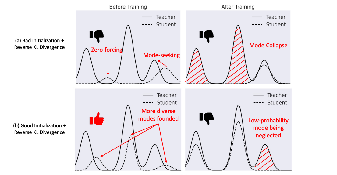
Figure 8: Mode collapse induced by the vanilla DMD reverse KL divergence term. Source: https://arxiv.org/abs/2507.18569

Indeed, our model struggles to generate complex camera motions. Samples taken from checkpoints earlier in the Self-Forcing training have many visual artifacts, but present much more dynamic camera motion.

Improved Distillation Objectives

There have been many improvements to the original DMD distillation techniques. Broadly, these can be divided into data-free approaches, requiring only sampling inputs like prompts, and data-driven approaches.

We believe the self-forcing approach of training on autoregressive rollouts is the most effective strategy to minimize the train-test mismatch in autoregressive video models. However, the DMD objective is a major target for improvement.

Techniques like Adversarial Distribution Matching for Diffusion Distillation improve upon DMD while remaining data-free.

Other approaches like DMD 2 expand on DMD by using real-world data and adding a GAN loss.

Autoregressive Adversarial Post-Training is another technique used to distill realtime autoregressive video models, and also performs train time autoregressive generator rollouts, but adds a GAN discriminator using real-world videos.

Task-Specific Models

Text to video is the most difficult task for a video model. Creating coherent temporal structure from pure noise is intuitively the most complex part of video generation.

For realtime applications that use a video as input, denoising from a partially noised latent rather than pure noise, the model gets this temporal consistency for free. For this specific task, it may make sense to fine tune the model only at lower noise levels. This makes the training task significantly easier and allows the model's full capacity to be used for its inference-time task.

The journey to Krea Realtime 14B was driven by a simple goal: to make generative AI a truly interactive creative partner. To achieve this, we tackled the fundamental engineering challenges that separate large, high-quality models from real-time performance. From developing memory-efficient training techniques at an unprecedented 14B parameter scale, to engineering a suite of novel inference strategies for stable, long-form generation, our work culminates in a model that responds at the speed of thought. By allowing users to guide and redirect video streams as they are created, Krea Realtime 14B represents a critical step away from "one-shot" generation and toward a future of fluid, collaborative, and controllable creative tools.

@misc{lightx2v,
  author = {LightX2V Contributors},
  title = {LightX2V: Light Video Generation Inference Framework},
  year = {2025},
  publisher = {GitHub},
  journal = {GitHub repository},
  howpublished = {\url{https://github.com/ModelTC/lightx2v}},
}

@misc{lin2025autoregressiveadversarialposttrainingrealtime,
  title={Autoregressive Adversarial Post-Training for Real-Time Interactive Video Generation},
  author={Shanchuan Lin and Ceyuan Yang and Hao He and Jianwen Jiang and Yuxi Ren and Xin Xia and Yang Zhao and Xuefeng Xiao and Lu Jiang},
  year={2025},
  eprint={2506.09350},
  archivePrefix={arXiv},
  primaryClass={cs.CV},
  url={https://arxiv.org/abs/2506.09350},
}

@misc{yin2024improveddistributionmatchingdistillation,
  title={Improved Distribution Matching Distillation for Fast Image Synthesis},
  author={Tianwei Yin and Michaël Gharbi and Taesung Park and Richard Zhang and Eli Shechtman and Fredo Durand and William T. Freeman},
  year={2024},
  eprint={2405.14867},
  archivePrefix={arXiv},
  primaryClass={cs.CV},
  url={https://arxiv.org/abs/2405.14867},
}

@article{huang2025selfforcing,
  title={Self Forcing: Bridging the Train-Test Gap in Autoregressive Video Diffusion},
  author={Huang, Xun and Li, Zhengqi and He, Guande and Zhou, Mingyuan and Shechtman, Eli},
  journal={arXiv preprint arXiv:2506.08009},
  year={2025}
}

I. Why the KV Cache has a Receptive Field > N

A Concrete Example

Consider a simplified setup where we generate a video frame-by-frame with a context window of 2 frames:

1. Generate Frame 0: Start with gaussian noise, denoise it with the transformer. Store Frame 0's keys and values at each transformer layer
2. Generate Frame 1: Start with gaussian noise for Frame 1. During denoising, Frame 1 attends to Frame 0's KV cache. Store Frame 1's keys and values at each transformer layer
3. Generate Frame 2: Evict Frame 0's keys and values. Initialize Frame 2 with gaussian noise, denoise with transformer

How Information Propagates Through Transformer Layers

The key insight is understanding what happens at each transformer layer when creating the KV cache:

Layer 0 (First Transformer Block):

• Frame 1's initial keys K₀ and values V₀ are computed via simple linear projection
• These K₀/V₀ contain only Frame 1's information
• No interaction with other frames yet

After Self-Attention in Layer 0:

• Frame 1 attends to Frame 0's cached keys and values
• The output is: Output = Attention(Q₁, [K₀, K₁], [V₀, V₁])
• Frame 1's hidden states are now a weighted combination that includes Frame 0's values
• This mixed representation becomes the input to Layer 1

Layer 1 (Second Transformer Block):

• Frame 1's keys K₁ and values V₁ are computed from the mixed representation
• These K₁/V₁ now contain information from both Frame 0 and Frame 1
• The information from Frame 0 has "leaked" into Frame 1's Layer 1 KVs

Deeper Layers:

• Each subsequent layer compounds this effect
• By layer L, Frame 1's KVs contain increasingly complex mixtures of all frames it has ever attended to

The Cascading Effect

When Frame 2 is generated with only Frame 1 in context:

• Frame 2 cannot directly attend to Frame 0 (evicted)
• But Frame 2 attends to Frame 1's KVs at all layers
• Since Frame 1's deeper-layer KVs contain Frame 0's information, Frame 2 indirectly accesses Frame 0's information

This creates a cascading effect where information from frames outside the current context window still influences the current generation through the stored keys and values.

Of course, one could argue that our solution—recomputing KVs from latent frames rather than evicting cached KVs—suffers from the same issue. Frames are produced by a transformer which has attended to previous frames' KVs, so this approach still technically has a larger-than-N receptive field. However, the keys and values from every transformer block are a far more expressive representation than latent frames and contain far richer information about evicted past frames.

II. Complexity of Block-Causal Masked Attention vs. KV-Cached Attention

Let us use the example of sampling frame-by-frame with 3 frames in context. Each frame contains S tokens.

For the regular self-forcing attention, we are performing attention between the S tokens of the most recent frame, and the 2 previous frames' tokens. S tokens attend to 3S tokens, giving a complexity of 3S²

With a block causal mask, the complexity is a sum of the attention costs for each frame block:

• Frame 0: Attends only to itself. Complexity: O(S²)
• Frame 1: Attends to itself and Frame 0. Complexity: O(S·2S)
• Frame 2: Attends to itself, Frame 1, and Frame 0. Complexity: O(S·3S)

The total complexity is the sum of these = 6S²

More generally, given N frames in context, we have:

O(S² · Σₖ₌₁ᴺ k) = O(S² · N(N+1)/2)

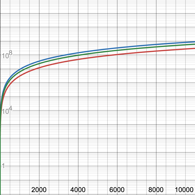
Figure 10: Log-scale graph of the computational complexities of different attention methods with N=3. Red: KV-cached self-forcing attention, green: block-causal attention, blue: full self-attention