Introduction
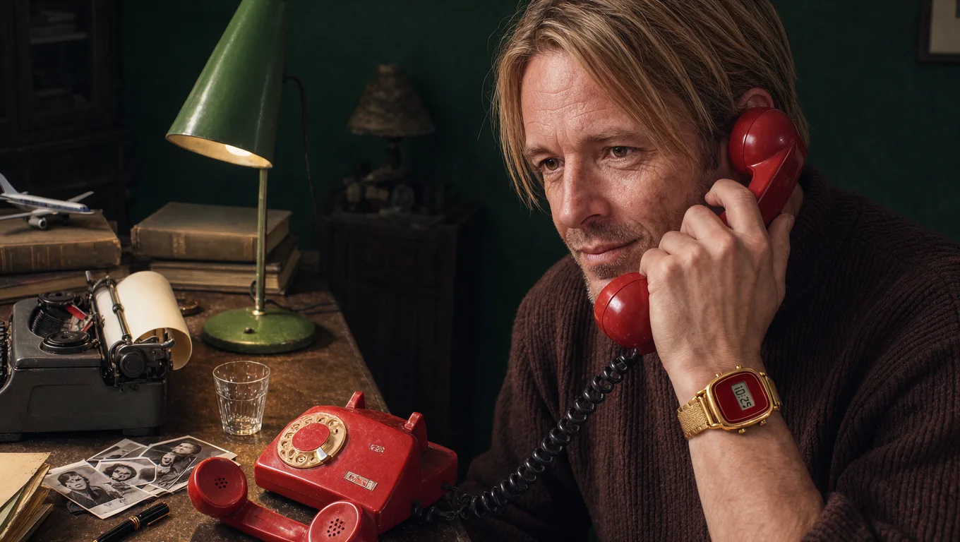
Text-to-image (T2I) models have transformed creative industries. However, while they have vast world knowledge, many visual tasks can’t be described with words alone. An identity, a product, or a design reference is easier to show than to describe. Image-to-image (I2I) models close this gap: they take reference images as input and reason over them alongside the instruction.
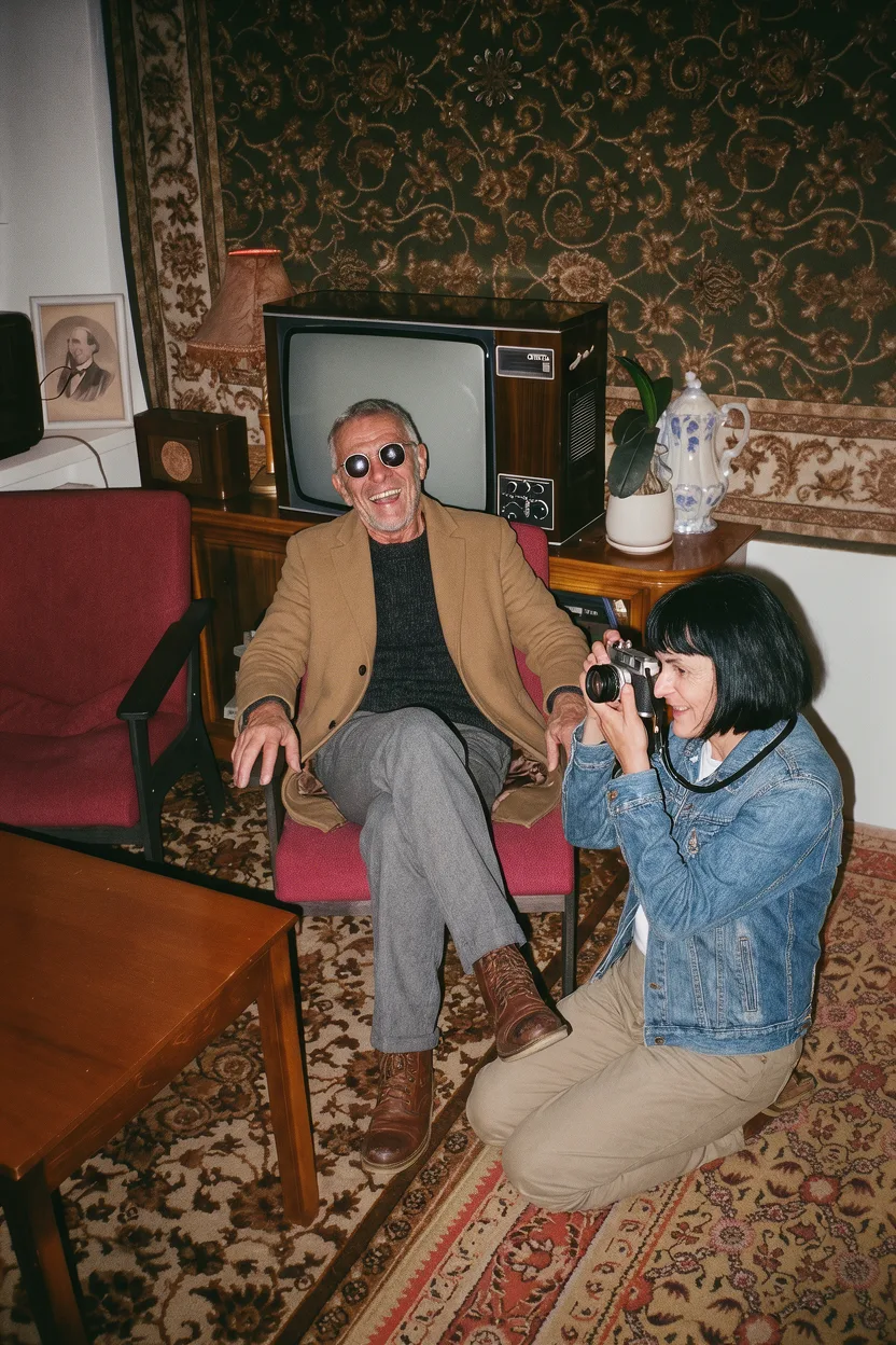
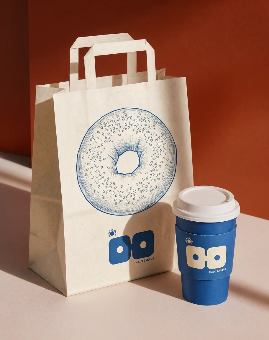
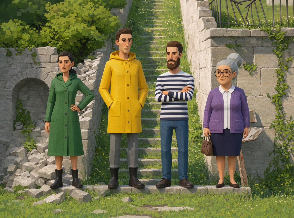
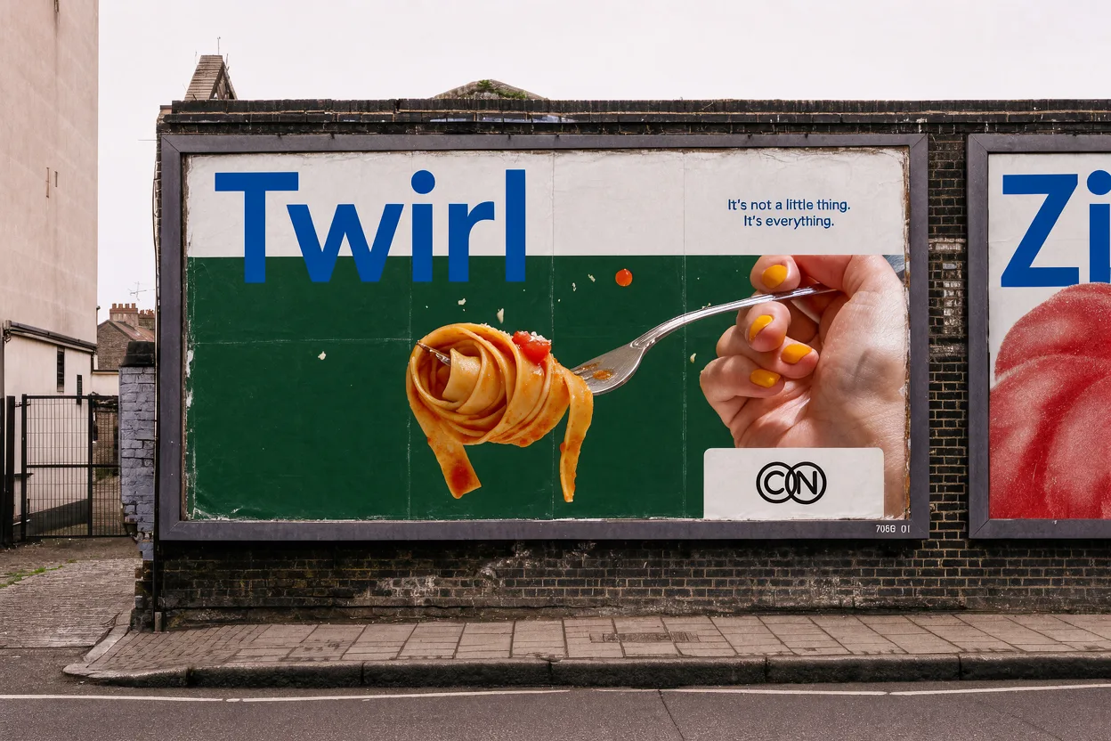
We introduce Krea 3, a foundation image-to-image model with frontier intelligence. It keeps characters and products consistent across edits, makes targeted changes while leaving the rest of the image untouched, and combines up to 8 reference images in a single generation.
However, a great creative tool is more than just an intelligent one. Frontier intelligence that takes minutes per image is unsuitable for professional creative work, where people try many versions of an idea before they keep one.
Once a model is smart enough to tackle complex tasks, the next frontier is speed and cost. Yet many recent image models have moved toward slower, more expensive generation in exchange for marginal quality gains.
Krea 3 takes the other side of that trade. It is an I2I model that is frontier quality, ultrafast, and cost-efficient.

Results
We compare Krea 3 against the I2I models that teams already use in production.
Krea 3 Ultra debuted at #4 on all independent arenas, making Krea the #2 image generation lab in the world, beating multiple trillion-dollar companies.
Arena
Multi-image edit
- 1 GPT-Image-2.5 Sunburst
- 2 GPT-Image-2.5 Flare
- 3 GPT-Image-2 (Medium)
- 4 Krea 3 Ultra
- 5 Gemini Nano Banana 2.1
- 6 Seedream 5.0 Pro
- 7 Muse Image
- 8 Gemini 3.1 Flash Image
- 9 Gemini 3 Pro Image Preview
- 10 Gemini 3 Pro Image (2K)
Artificial Analysis
AA-Image-Editing v2.1
- 1 GPT Image 2.5 Sunburst (max)
- 2 MAI-Image-2.7-Preview
- 3 GPT Image 2.5 Flare (max)
- 4 Krea 3 (Ultra)
- 5 Nano Banana 2.1
- 6 MAI-Image-2.6
- 7 MAI-Image-2.6-Flash
- 8 GPT Image 2 (high)
- 9 Seedream 5.0 Pro
- 10 Muse Image
Design Arena
Image editing
- 1 GPT-Image-2.5 Sunburst
- 2 GPT-Image-2.5 Flare
- 3 GPT Image 2
- 4 Krea 3 (Ultra Thinking)
- 5 Reve 2.0
- 6 Reve 2.1
- 7 ChatGPT Image
- 8 Grok Imagine Image 2 A…
- 9 Muse Image
- 10 Grok Imagine Image 2…
Figure 1: Arena.ai, Artificial Analysis, and Design Arena image-to-image leaderboards.
Figure 2: Quality vs. speed. Elo measured from the Artificial Analysis Image Editing benchmark.
Speed is where Krea 3 differs most. In production, Krea 3 finishes edits within 8s. In our production traffic, Nano Banana Pro takes around 20 to 40 seconds for a comparable edit, which makes Krea 3 roughly 3–5 times faster. The gap widens even more when compared against GPT Image models, which can take up to several minutes to perform an edit.
Figure 3: Mean latency of I2I models with one reference at 2K output, the most common setting on our platform, measured through the fal API.
While maintaining competitive performance against models such as Nano Banana Pro and GPT Image 2, Krea 3 brings significant cost efficiency to the table, allowing users to access fast, high-quality editing capabilities at a fraction of the price.
Figure 4: Monthly cost of 100,000 edits for each I2I model, at API prices.
Architecture
Our architecture is deliberately standard; the contributions of this work are in training, data, and post-training. We initialize Krea 3 from the Krea 2 [1] pretrain and continue pretraining on a significantly wider and improved text-to-image dataset, including native 2K resolution samples. We then introduce image-to-image data and extend the text-to-image architecture as follows:
- VAE-encoded reference images are injected into the DiT image stream. Reference images are encoded with a variational autoencoder (VAE) [2] and appended as clean tokens to the diffusion transformer (DiT) [3] latent image sequence using timestep modulation vector
t = 0. This choice of timestep modulation is in-distribution at initialization, as the reference tokens are always clean. Also, removing timestep dependence enables later causal distillation, allowing key–value (KV) caching of the reference image tokens. - Edit instruction tokens attend to VLM vision tokens. Krea 3’s text encoder is a vision-language model (VLM), so we feed it the reference images (downsampled to a 384² pixel area) alongside the edit instruction, letting instruction tokens attend to reference image tokens inside the VLM. Only the instruction tokens are passed to the DiT; the vision tokens are dropped, since the VAE latents contain a higher-fidelity version of the pixel information.
Thus, the final DiT inputs are:
- edit instruction tokens (that have attended to VLM vision tokens)
- clean reference image VAE latents
- noisy VAE target latents
Hover or tap a block to trace its path through the model.
Figure 5: Krea 3 image-to-image diffusion transformer architecture.
Training
Training a large transformer on image-to-image data with variable reference counts and resolutions required three systems changes: decoupled reference–target resolution sampling, length-binned packing, and sequence-length-dependent memory optimization for native 2K training. We describe each below, along with the timestep-shift tuning that most improved structural coherence.
Decoupled reference-target resolution
During training, we sample the pixel area of every image in a row independently: the target and each reference get their own resolution.
Decoupling reference and target resolutions is important for inference-time flexibility. Some tasks need high reference fidelity; copying fine text, for example, requires seeing the reference at high resolution. Others, like placing a simple product, don’t need as much detail preservation. In these cases, pairing a high-resolution output with lower-resolution references shortens the sequence and speeds up sampling with little to no quality loss.
Length-binned packing with native aspect-ratio training
For a given training row, the DiT’s sequence length is the sum of:
- edit instruction tokens: depends on the length of the edit instruction
- reference image tokens: depends on the number of reference images and their resolutions
- target image tokens: depends on the target resolution
For training efficiency, all ranks must process homogeneous sequence lengths. This is challenging in image-to-image training because the dataset contains a wide range of reference image counts and resolutions.
Edit instruction tokens are always padded to a fixed maximum length.
For image tokens, we create a resolution plan once per epoch. At the start of the epoch, we sample a resolution for every reference and target image in the dataset from a fixed set of training resolutions. This plan determines the sequence length for every row in the dataset for the current epoch.
On every train step, we sample:
- a reference image count
- a token length from a set of discrete token lengths
These two values are shared by all ranks. The dataloader yields training rows with the sampled number of reference images, at or below the sampled token length. Any shorter samples are padded to the token length bin (Figure 6).
Figure 6: Length-binned packing per training step. All ranks in a step share one bin and one reference count.
A global reference count isn’t strictly necessary for the transformer, but it keeps VLM computation homogeneous across ranks, so we sample one per step.
Because homogeneity comes from the token-length bins rather than aspect-ratio bucketing, we can train on references and targets at their native aspect ratios (including exotic ones) with minimal cropping.
Native 2K training
Krea 3 significantly improves text rendering over Krea 2, primarily from scaling to native 2K. The bottleneck at lower resolutions is lossy VAE compression: at 1K, fine text does not survive an encoder–decoder round trip, so the model cannot learn to render it. At 2K, the image is large enough for text to be represented and learned. The same effect benefits overall aesthetics and fine textures: detail like fabric, hair, and skin that is lost at 1K stays intact at 2K.
Scaling to 2K makes sequence length explode in multi-reference editing. A 1024×1024 text-to-image sample uses 4,096 image tokens; a 2048×2048 target with seven 2048×2048 references uses 131,072, 32× as many.
Sequence-length-dependent memory optimization
To handle these long sequence lengths under GPU memory constraints, we use context parallelism, Fully Sharded Data Parallel (FSDP) sharding, gradient checkpointing, and bfloat16 (bf16) AdamW moments.
Most of these slow training: context parallelism shrinks the per-step batch and requires gradient accumulation, and gradient checkpointing adds recomputation. They’re necessary for long sequences but overkill for low-resolution, low-reference rows, so we tune them per sequence length, adjusting batch size and which blocks are checkpointed so short rows aren’t slowed down.
Timestep shifting
We carefully analyze the denoising trajectories of intermediate models throughout training to tune the train-time noise schedule shift.
Figure 7: Denoising trajectory of a multi-reference edit; global structure is planned at high noise levels.
We find that most of the global structure, especially on complex multi-reference tasks, is decided at high noise levels. Unlike other implementations, which use the same timestep shift [4] for text-to-image and image-to-image, we use a more aggressive timestep shift for image-to-image, concentrating training and inference steps at high noise levels. In our ablations, this choice significantly improved structural coherence and accelerated convergence.
Data — from pretraining to supervised finetuning
Data for pretraining and supervised finetuning (SFT) shares the same pipeline and philosophy, so we describe it together here. The data for reinforcement learning (RL) and Direct Preference Optimization (DPO) is discussed in their respective sections.
Data philosophy
From pretraining to SFT, training samples consist of:
- a target image
- one or more reference images
- a text instruction describing how to produce the target, given the references as context
We can define a good training sample as one where:
- The target image meets aesthetic and quality standards.
- The reference image(s) provide useful visual context that the generative model can use to produce the target image.
- The edit instruction captures all the dependencies between the target image and the references, as well as any novel elements of the target that don’t come from the references.
Essentially, the visual information from the reference images and the edit instruction should together be comprehensive enough to perfectly represent the target image. For example:
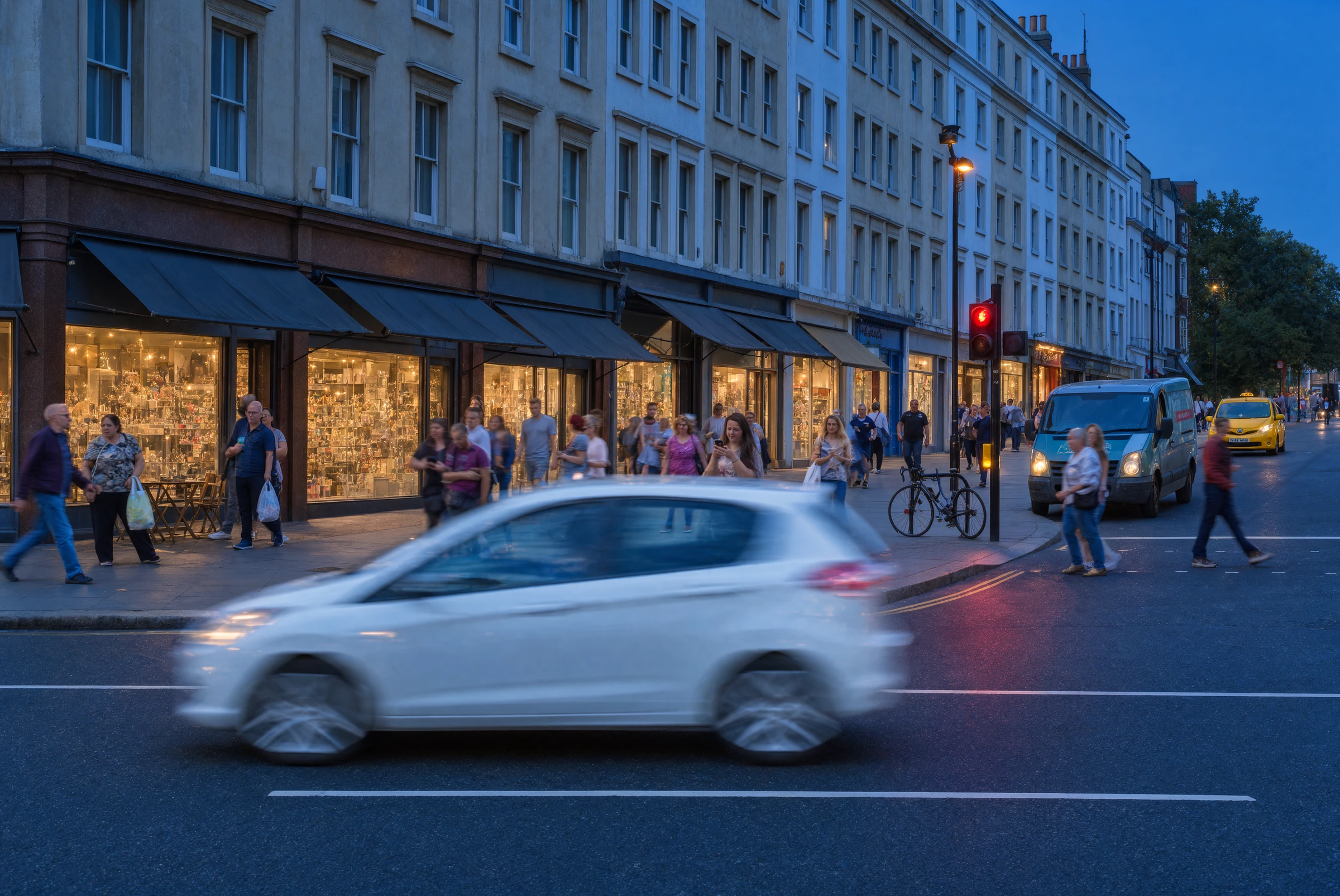
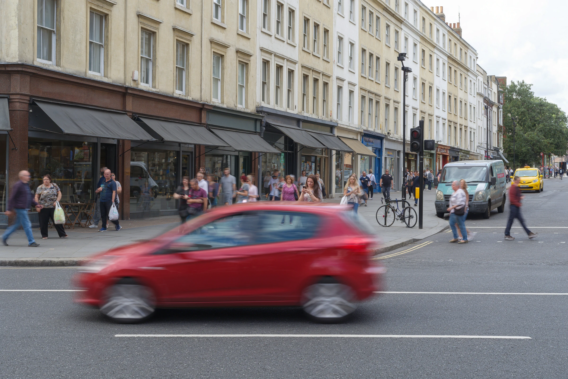
In <image-1>, the motion-blurred hatchback crossing the foreground is white instead of red, keeping its shape, blur and position. The whole street is shown at blue hour: the sky is a deep twilight blue, the facades and road take a cool dim blue ambient light, and the shop windows, the street lamp on the pole and the red traffic signal glow, their light reflecting on the white car's body and the asphalt. The pedestrians, buildings, van, taxi and camera are as in <image-1>.
Figure 8: A training sample in which the reference and the instruction together fully describe the target.
The instruction spells out what to keep from the input (scene and composition) and what to change (lighting, time of day, car color).
Domain balancing
Image-to-image tasks vary widely in what must change and what must be preserved from references. We define two broad categories, local edits and novel generations, which we further break down into a fine-grained taxonomy for dataset balancing.
Local edits
Local edits require parts of a reference image to remain structurally identical or unchanged at the pixel level. Changing part of a label while leaving the rest of the image untouched is one example.
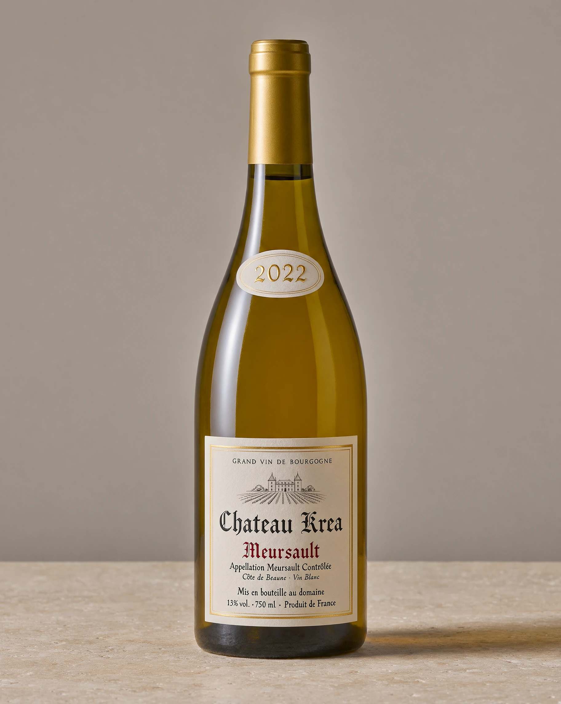
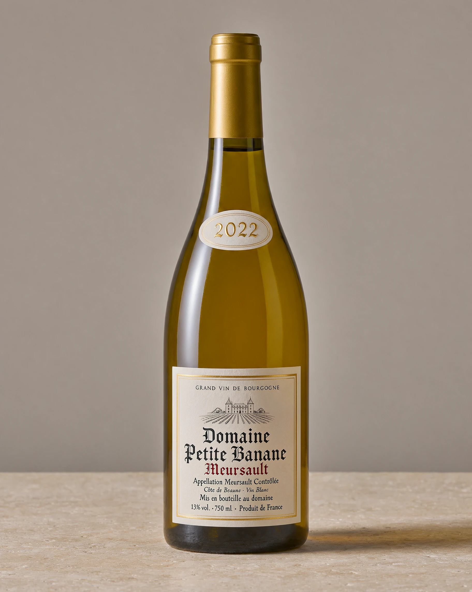
In <image-1>, the two-line estate name “Domaine Petite Banane” on the label reads “Chateau Krea” on a single line, in the same black blackletter type. The rest of the label, the bottle, the lighting and the background are as in <image-1>.
Figure 9: A local edit that rewrites the estate name on the label and leaves the rest of the image unchanged.
Novel generations
Novel generations use reference images as visual context, but their outputs are fundamentally novel images, not localized edits to one of the references.
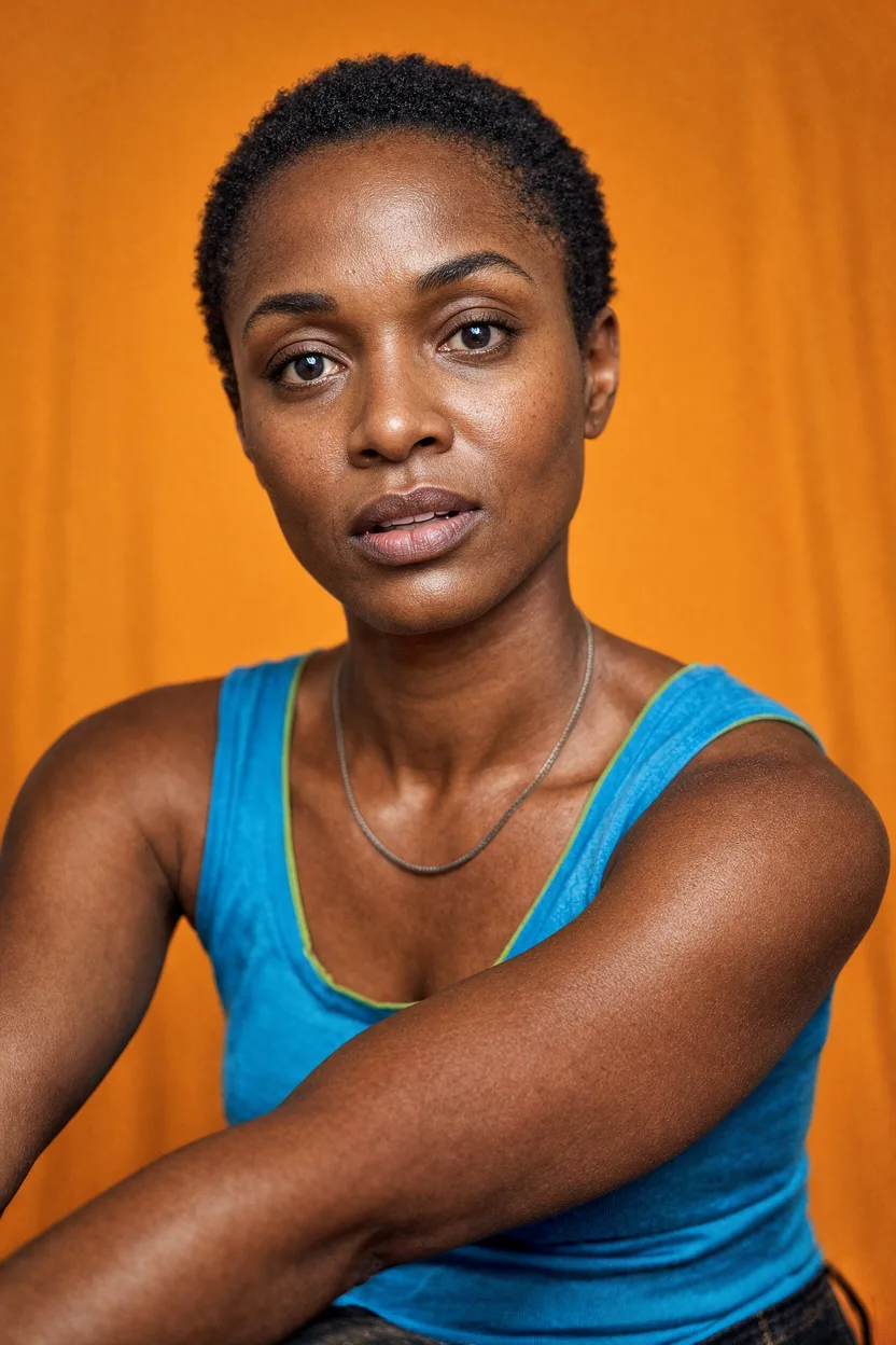
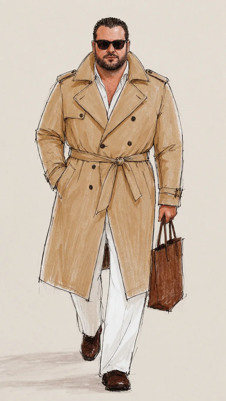
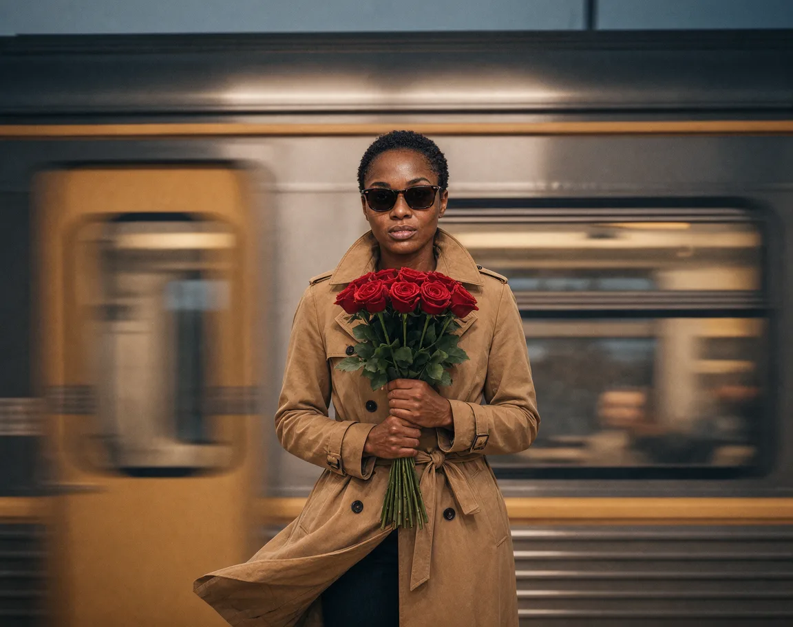
Show the woman from <image-1> wearing the coat and sunglasses from <image-2>, holding the same red roses with the train passing behind her.
Figure 10: A novel generation that puts the woman from one reference in the coat and sunglasses from another, in a new scene.
Mining image-to-image data from massive unstructured data
One of the most effective strategies is to mine related images from our existing pretraining image pool, which contains billions of images. The pool naturally contains related images which we can use to create image-to-image pairs. For instance, famous landmarks like the Eiffel Tower have been photographed thousands of times under different conditions. We use efficient embedding models to retrieve images that are similar but not identical, and use a cascaded VLM pipeline to audit the quality of candidate pairs.
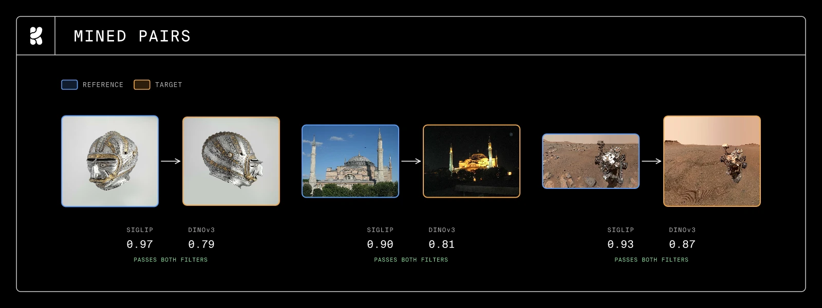
Figure 11: Same-subject editing pairs mined from billion-scale unstructured data with our pipeline. All images shown are CC0 or public domain.
We use a multi-model pipeline, including LoFTR [5], SIFT [6], DINOv3 [7] and SigLIP 2 [8] similarity, and the Qwen family of VLMs. We manually tune the thresholds and criteria in our filtering pipeline to find optimal domain-specific heuristics. For example, photorealistic images that share high DINO classification (CLS) token similarity but have patches of low DINO similarity often make good image pairs, i.e., the high-level semantics of two images are similar (a shared subject), while their localized content differs (in camera angles, time of day, subject, etc.).
Our initial pool of images already has high-level metadata about domain, and we tune the filtering pipeline according to domain, dropping, for example, face embeddings and LoFTR for non-photorealistic domains where they perform less well. We also tune the similarity thresholds for the SigLIP 2 and DINOv3 models for different domains (photorealism, illustration, etc.).
We then use a multi-stage VLM filtering pipeline to audit these candidate training rows for quality. During this stage, we are not trying to produce the edit instruction, because computationally cheap models are not reliable enough to capture the level of precision we want. Rather, our goal is to validate that there is a clear relationship between the reference image(s) and the target image, such that an image model can learn to use the references’ visual content as context for generation.
- CANDIDATE PAIRS SigLIP 100%
- DINOv3 ×0.45
- VLM FILTER Qwen3.5 9B ×0.047
- VLM AUDIT Qwen3.6 27B ×0.45
- DEDUP SigLIP ×0.18
- IMAGE PAIRS 0.17%
Figure 12: The multi-stage pipeline for mining image-to-image pairs from unstructured data.
After gathering candidates based on SigLIP 2 similarity and the per-domain heuristics mentioned above, we apply a DINOv3 CLS-token filter to the candidate pairs, keeping 45%. We then use Qwen3.5-9B [9] to validate whether the pair can be made into references and targets that are related enough to train on, which keeps approximately 4.7% of the pairs it processes. A larger, more intelligent VLM, Qwen3.6-27B, audits the remaining pairs and retains ~45% of them. Finally, target-image-level deduplication keeps 18% of the remaining rows.
From the initial pool of SigLIP 2 candidate pairs, 0.17% of pairs survive all four stages.
Because the majority of the candidate pairs are filtered early by cheap embedding models, this pipeline is tractable to run, even at our scale of billions of images. We run these embedding and VLM filtering jobs as low-priority workloads on our cluster, which schedules on any idle compute.
Mining image-to-image data from natural groups
Embedding models are good at finding very visually similar images. However, they struggle to find rows where references and target share a strong high-level semantic connection without looking visually similar. For example, an architectural floor plan and a cutout rendering of the completed building would form a strong training pair for a complex task, but would be dropped by the above pipeline.
Some real-world images are naturally grouped into galleries, albums, or collections by the same author. Images within these groups are likely to share the high-level semantic connections needed for such training pairs. For example, a Wikipedia page might contain several closely related images whose connection an embedding model alone would miss.
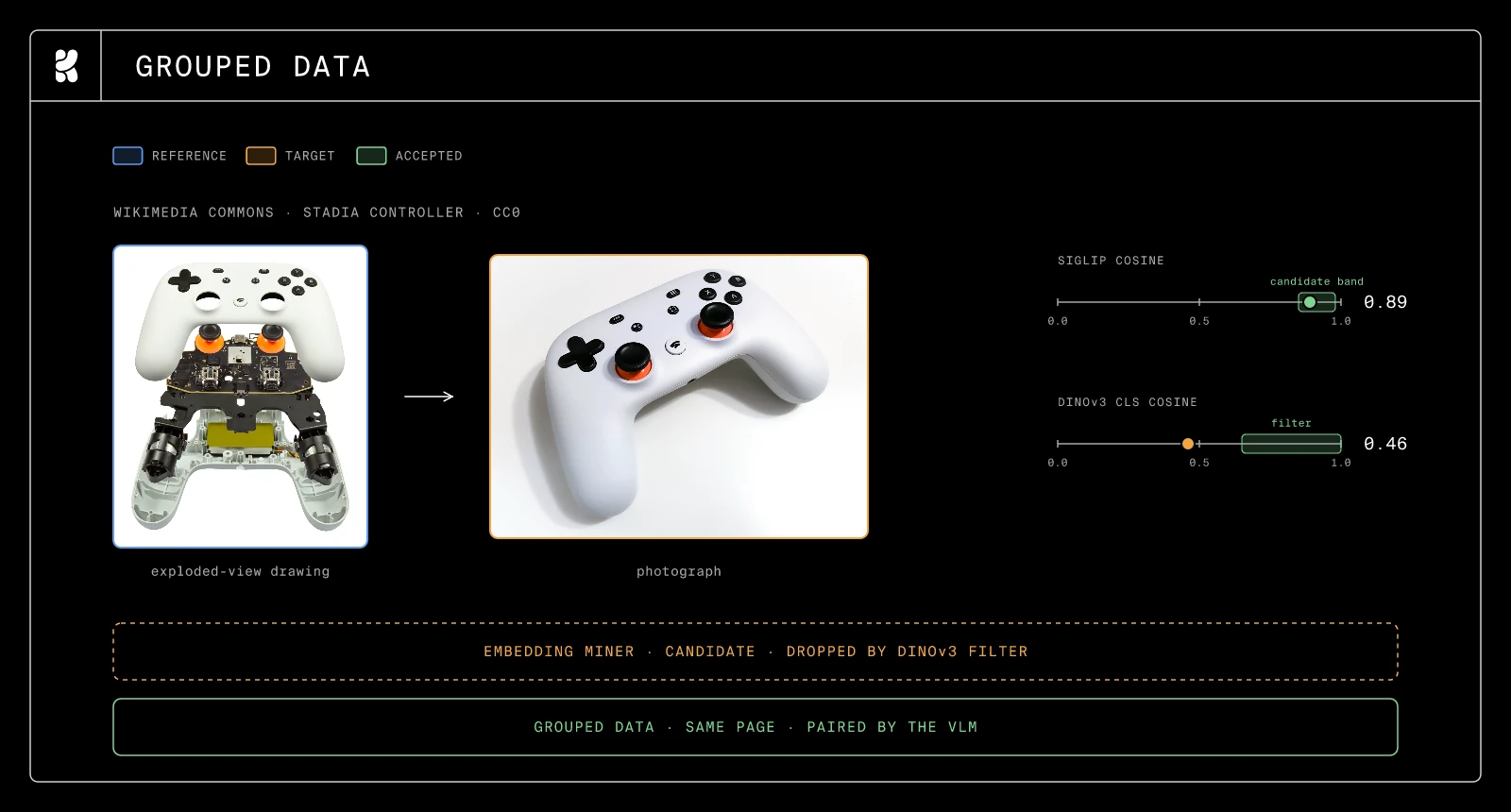
Figure 13: A strong editing pair our embedding pipeline would drop, recovered by running a VLM directly on a grouped source. Source: Wikipedia.
We use a VLM-based pipeline to extract the highest-quality images from such natural clusters to use as targets and select the most suitable references from the remaining images. This pipeline is an especially strong source of multi-reference data.
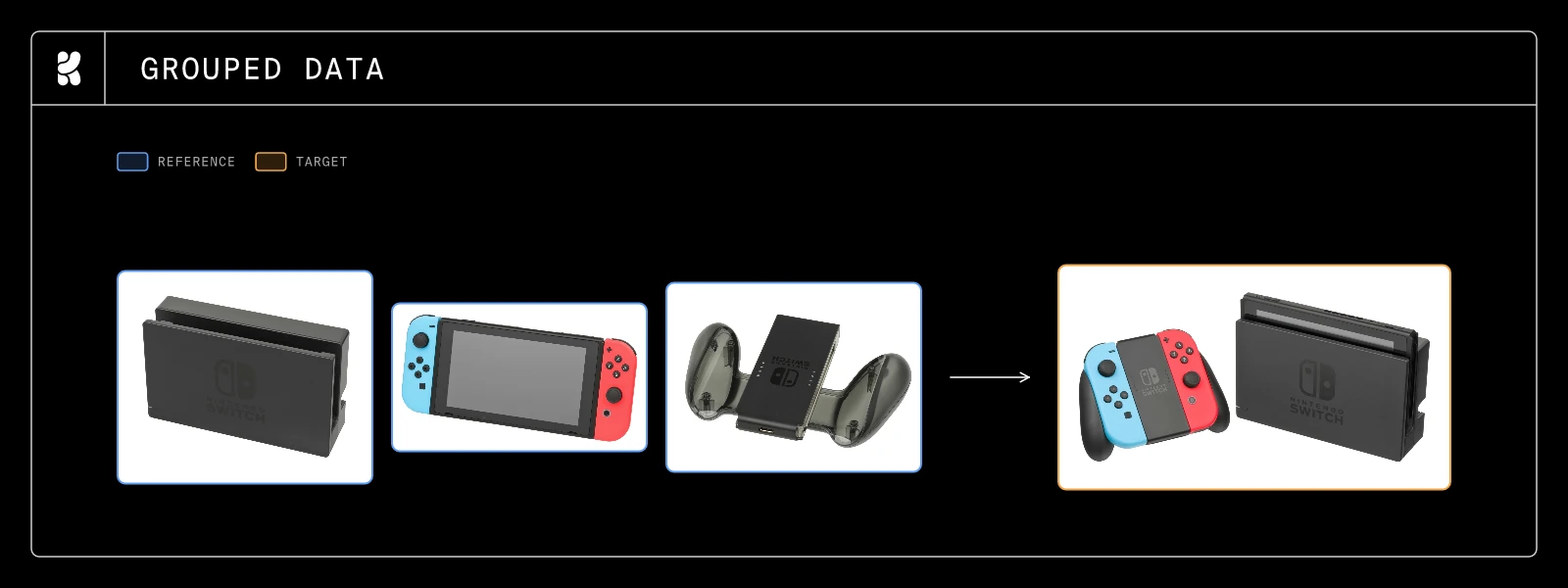
Figure 14: A strong editing multi-reference training row, mined by passing multiple images from a naturally grouped source into a VLM pipeline that can select multiple references.
Synthetic data
In addition to mining image-to-image training rows in the wild, we generate synthetic training pairs, where we perform the edit ourselves, so we know exactly what changed between reference and target.
Some pairs are fully rendered. We render websites with modified text and Cascading Style Sheets (CSS) to improve precise local edits, and render novel viewpoints of ground-truth 3D scenes to improve novel view synthesis. When captioning these pairs, we pass ground-truth metadata about what edit was performed to the captioner to prevent caption hallucinations.
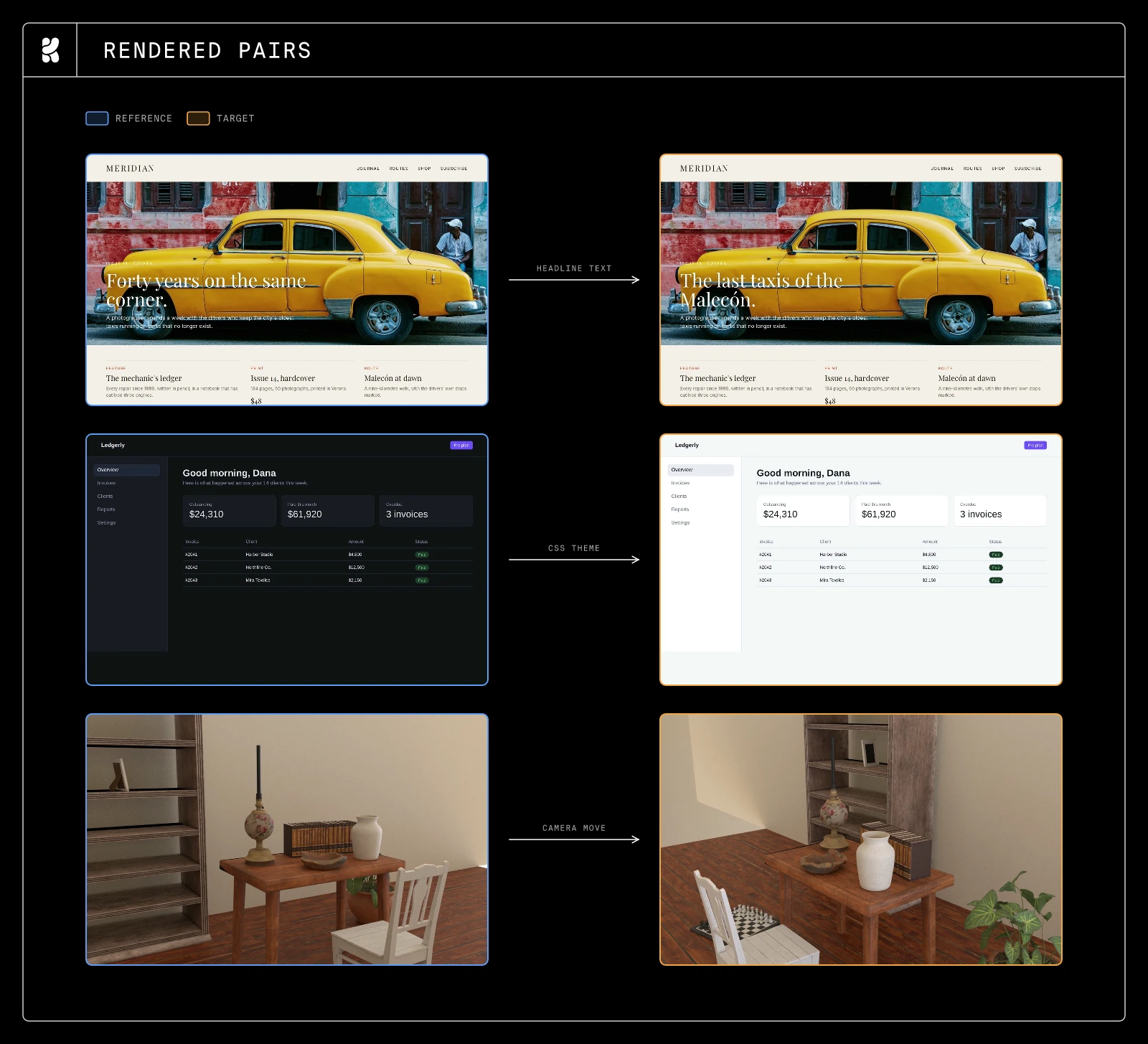
Figure 15: Synthetic training samples generated by making ground-truth edits to website HTML, CSS, and camera positions in 3D scenes.
Other pairs start from a real image and apply a transformation with a known result. Many editing tasks map onto standard computer-vision tasks: to learn depth-to-image, we run a depth model on a real image; to learn pose- or structure-conditioned edits, we run ControlNet-style [10] annotators to extract a skeleton or edge map. Each real image yields an image-to-image pair at almost no cost, and we can also augment conventional pairs with the target’s structural conditioning. Tasks like inpainting and outpainting are trivial to synthesize and teach faithful preservation of unedited regions.
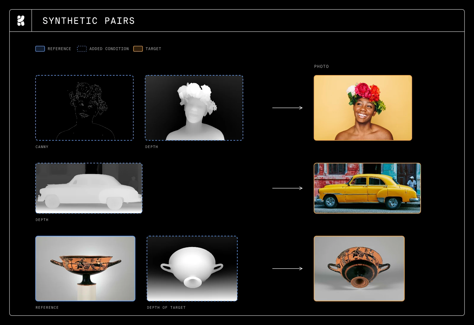
Figure 16: A cheap vision annotator (Canny / Depth) turns any real image into an image-to-image training row.
Designing the conditioning
The above pipelines yield image data with vast domain coverage. However, while world knowledge comes from image data diversity, the model’s intelligence comes from high-quality instruction conditioning.
VLMs often fail to produce accurate edit instructions for training. The most common failure cases are:
- omitting changes between references and target
- hallucinating changes that never occurred
- failing to include output text verbatim in double quotes
- ignoring one or more references and focusing on a subset of the reference images
Training on such flawed captions teaches the model to make unwanted changes at inference time and degrades its overall instruction following.
The perfect edit instruction is a comprehensive recipe that turns the reference image(s) into the target. It leans on the reference images where they provide visual context and fills in the gaps where they do not. Given two photos of the same building, the instruction must describe every change, so that the model never learns to perform edits the prompt did not request. This is harder than it sounds: captioners often omit smaller changes, like a subtle camera-angle shift, when a large one, like a change in time of day, dominates.
Training on short prompts is tempting: it would let the model handle terse user requests by learning implicit edits. But in our ablations, models trained on a mix of long and short prompts performed worse than models trained on long prompts alone, even when evaluated on detailed prompts. The failures of short prompts are especially visible when rendering text. In short prompts where the text is implicit (e.g., the prompt “a photo of a sign that describes rocket science”), the model fails to generate coherent text. But when text is explicitly spelled out in a longer prompt, the model can render it faithfully. Training on and inferring with detailed prompts solves this problem.
To produce captions that meet this bar, our captioning pipeline uses structured reasoning. Before writing the final caption, the captioner must produce:
- a comprehensive optical character recognition (OCR) pass, outputting all text in the target image
- an exhaustive global caption of the target image
- a dependency section attributing every aspect of the target that comes from a reference image
- an explicit diff: every change between the references and the target
By forcing the captioner to structure its output like this, we help it produce final captions that meet our requirements, substantially reducing hallucinations, misattributions, and omissions.
Text-to-image regularization
To preserve the model’s text-to-image prior, we train on a 30:70 blend of text-to-image and image-to-image data. The T2I fraction maintains the model’s generative ability and mitigates aesthetic degradation from I2I training. We ablated this ratio: less T2I data caused structural and aesthetic degradation, while more slowed I2I convergence without improving quality.
Supervised finetuning data
SFT uses the same definition of a good training sample as above; what changes is how strictly we curate. We tighten the quality bar with more stringent filters, handpick sources for aesthetic quality, and employ more expensive VLM filtering pipelines.
We make one deliberate exception here. We do not filter on reference-image quality, so the model learns to produce aesthetic outputs even from low-quality references.
Beyond quality filtering, we balance the data toward tasks the model struggles with. We identify weaknesses through VLM judges and visual inspection and curate task-specific datasets, for example for multi-identity preservation.
We also make tasks harder by limiting the input context. Our e-commerce data, for instance, contains samples with multiple views of a product as input images; during SFT, we upweight rows where the input is cut down to the minimum viable context needed to produce the target.
Reinforcement learning
Pretraining and SFT equip Krea 3 with world knowledge and its general editing ability, but the model still makes mistakes. It occasionally misspells words, modifies parts of the references it was asked to preserve, and ignores parts of the instruction. The goal of reinforcement learning (RL) is to improve the reliability of the model, not to give it new capabilities.
Using our taxonomy of I2I tasks, we curate challenging inputs across various domains. We carefully filter them offline so that no input is too hard or too easy at the start of an RL run. We design multiple task-specific rewards and use an agentic harness to select appropriate rewards for each training input.
During an RL run, the model generates a group of 16 rollouts for each input, and each rollout is scored by a per-input set of rewards. We compute the group-relative advantages [11] and use DiffusionNFT [12] for the policy update.
Agentic reward harness
We preprocess our RL dataset with an agentic VLM harness. This harness determines the success criteria for a given input and selects the rewards that verify them (Figure 17).
Offline · once per training input
paraphrases · instruction · plans
Hover or tap any block, plan or reward to trace what it feeds.
Figure 17: Overview of the RL pipeline, with the offline agents above and the online RL step below.
Before training, the planner agents read each training input and produce up to three plans:
- a rubric of fine-grained requirements that the output must satisfy.
- a text plan that lists every string the output must render, keep, or remove, if the output image contains text.
- a region plan that marks the edit region with bounding boxes, if the generation is a local edit.
These plans determine which rewards will be used to score the rollouts. The next three sections describe how these rewards are implemented.
General rewards
Pointwise rubrics: judging rollouts individually
A natural reward design for general edits is a rubric [13, 14, 15, 16]. A rubric is a comprehensive list of binary checks generated from the instruction and reference images, such as “the hat is on the dog” or “the dog’s pose is unchanged”. Rubrics provide useful signal, but a pointwise rubric judge is easy to saturate. By the end of an RL run, about 70% of rollouts score a perfect 1.0, and more than half of the groups have zero reward variance, providing no learning signal (Figure 18).
Figure 18: A pointwise rubric judge saturates over an RL run.
Pairwise rewards: comparing rollouts within a group
We therefore add two pairwise rewards. Instead of judging rollouts in isolation, a judge sees two rollouts from the same input and selects a winner. A preference judge says which edit better does what was asked, and a rubric judge goes through the rubric and says which one better satisfies each requirement. Given the same rubric, the comparison agrees with human preference far more often than pointwise scoring does.
Pairwise verdicts are also more stable than pointwise ones. VLM judges are stochastic, and when we asked our pointwise judge a second time, 43% of the pairs it had ordered within a group flipped. Pointwise scores are so saturated that a small change in the judge’s answer can reverse the ranking within a group, and converting rewards into advantages then amplifies these small differences. Pref-GRPO [17] reached a similar conclusion for text-to-image RL. A pairwise design avoids most of this, because both rollouts are judged in the same call against the same bar.
There are many different ways to convert a pairwise signal into a scalar per-rollout reward (Figure 19). In a full round robin, where every pair of rollouts is compared once and each rollout is scored by its wins and losses, the judging cost would scale quadratically with the group size. Cheaper alternatives fall short in other ways, as random pairs are prone to “lucky draws”, where a rollout scores higher only because it met a weaker opponent, and a knockout bracket only finds the winner and leaves the first-round losers unranked. We implement a simple solution where we randomly designate one rollout as a “pivot” and compare every other rollout against it. Because every rollout faces the same opponent, the share of a rollout’s score variance that comes from its opponent falls from 25% with random pairs to 4%, and at about the same number of judge calls the pivot’s ranking comes closest to that of the full round robin.
to train with 1.00 120 judge calls at n = 16
inflates a score 0.69 16 judge calls at n = 16
stay unranked 0.44 15 judge calls at n = 16
the same opponent 0.74 15 judge calls at n = 16
Figure 19: Four ways to pair n rollouts, and how well each ranks them at n = 16.
Catching visible defects. Alongside the pairwise rewards, we add a defect judge, which looks at each rollout on its own and searches only for visible defects, such as pasted-in elements with the wrong scale or lighting, broken anatomy, or regions that look cut from different photos. Hong et al. [18] find that text-to-image RL policies can learn such artifact-prone images while still scoring well, and use an artifact reward to regularize training.
Text rewards
Text rendering is one of the most important image-to-image tasks and is highly verifiable. It was also the task where our initial reward design failed the most often.
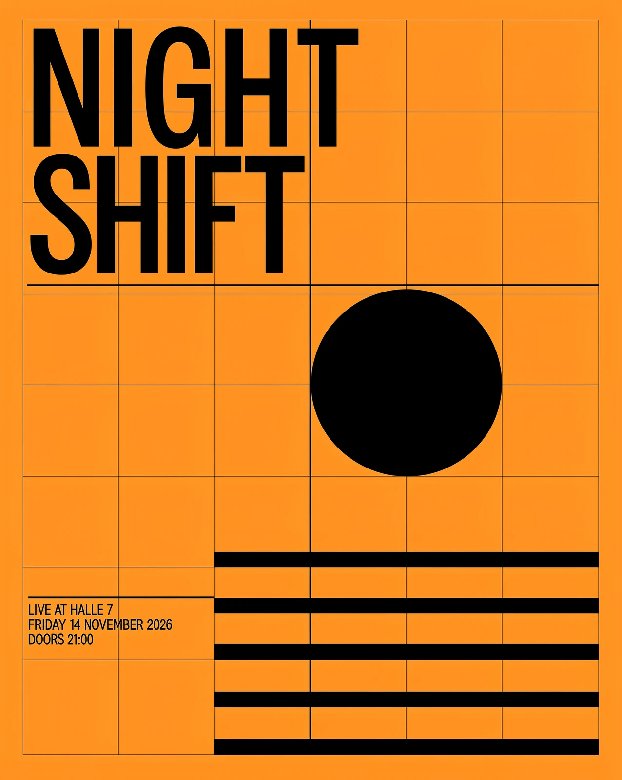
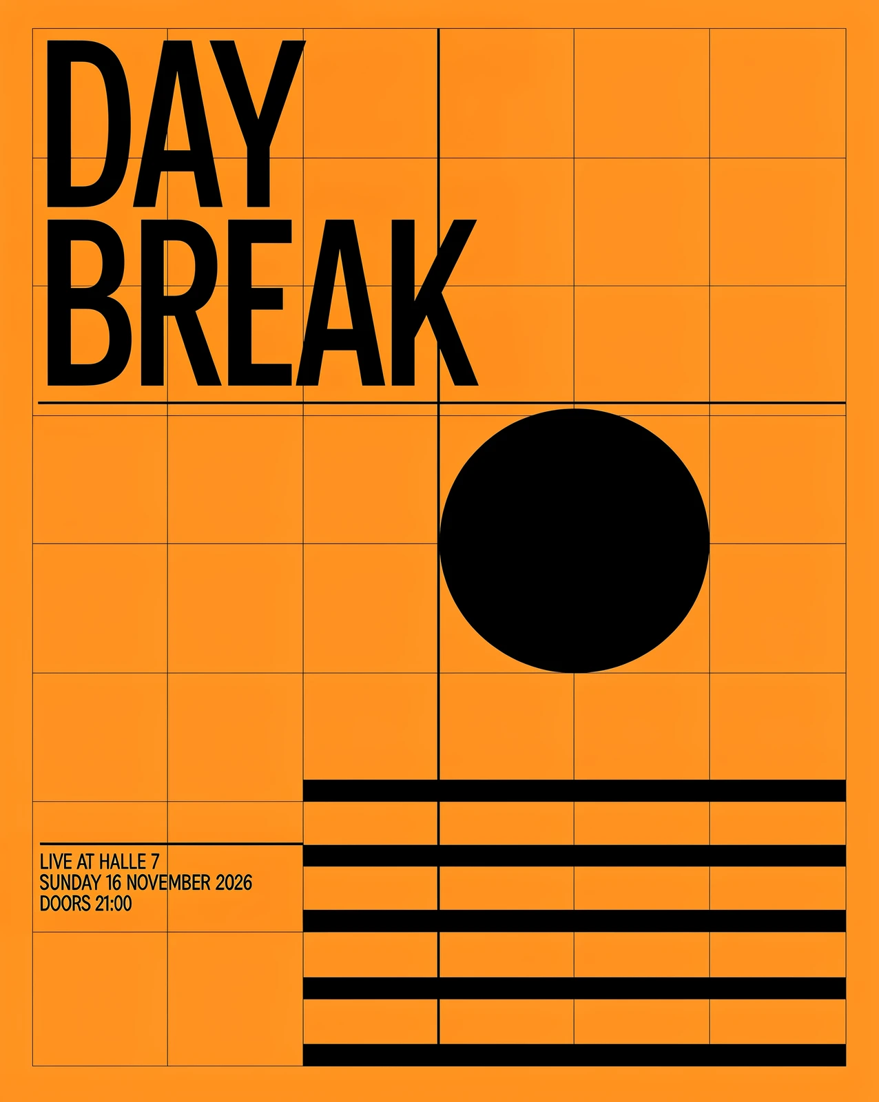
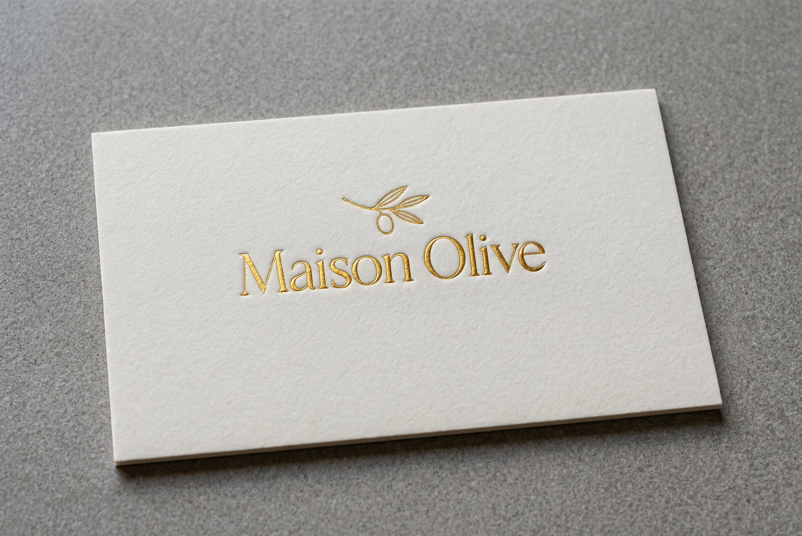
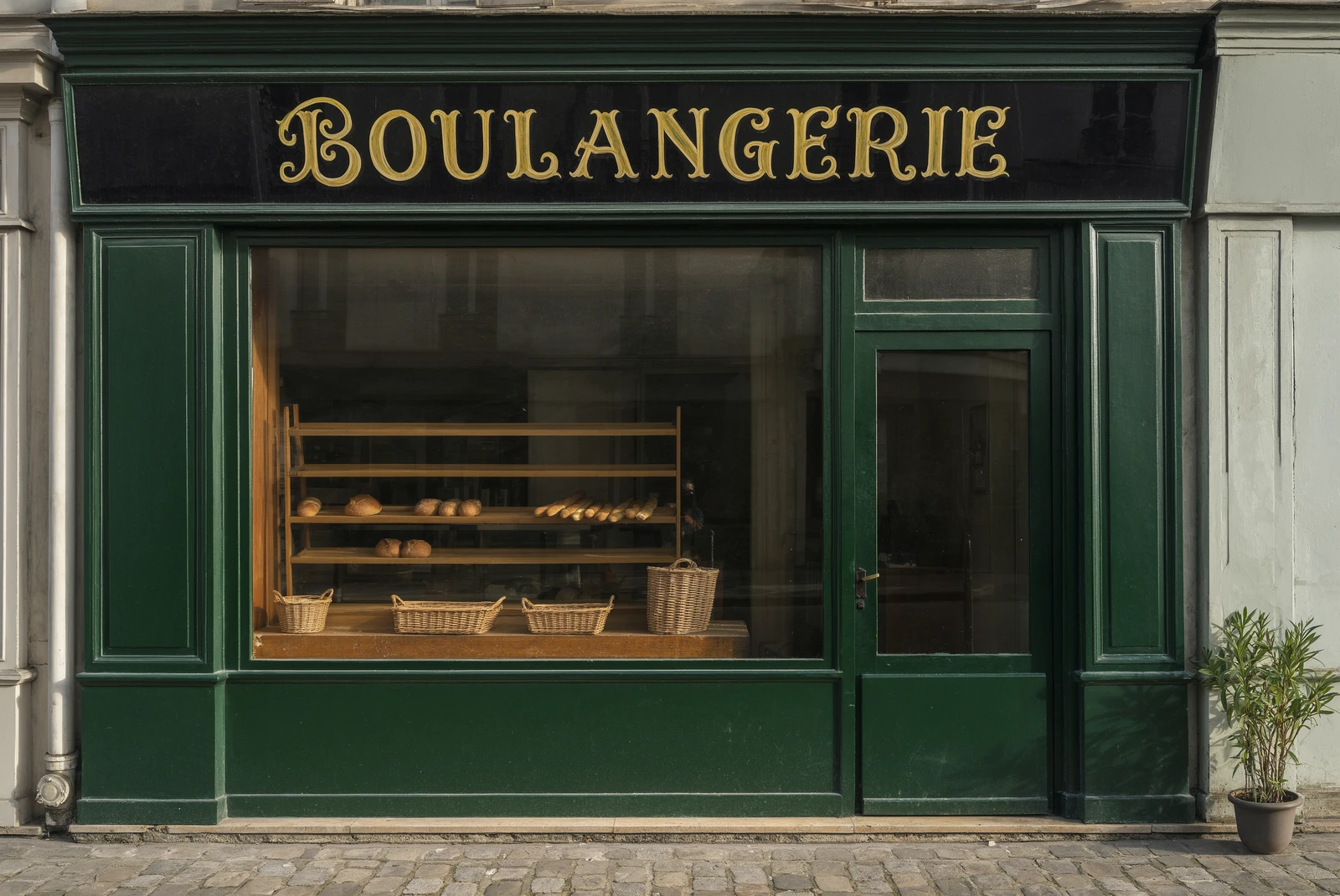
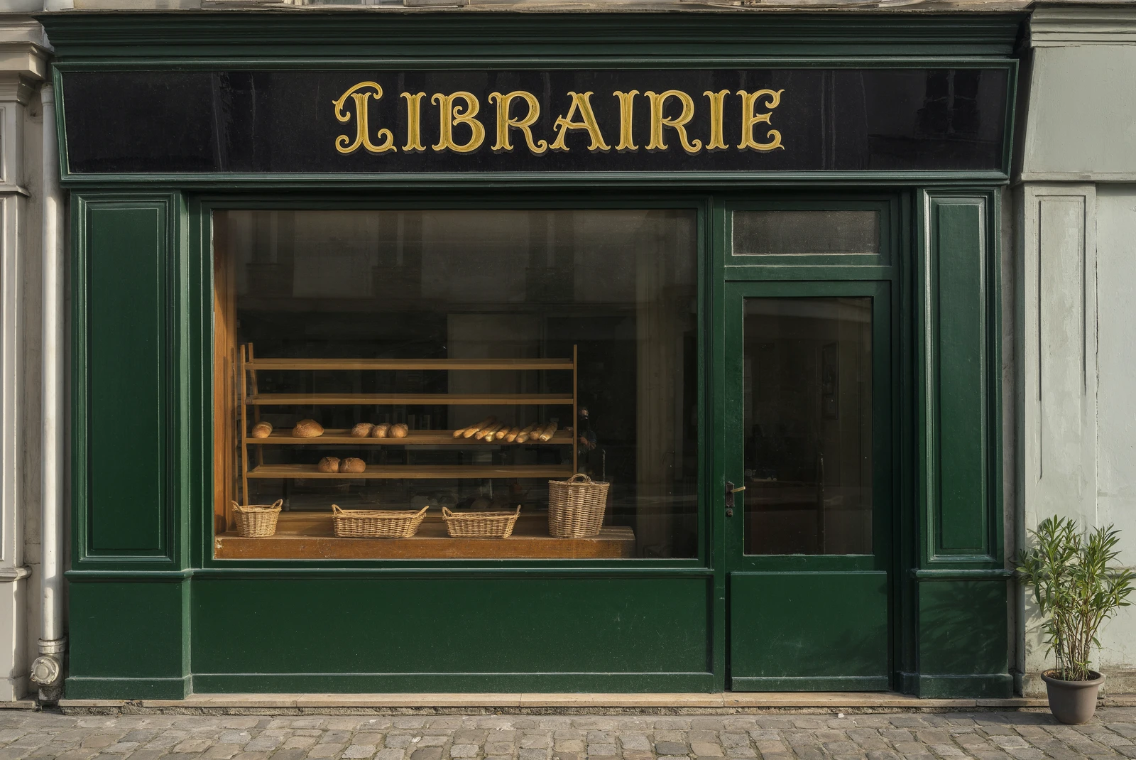
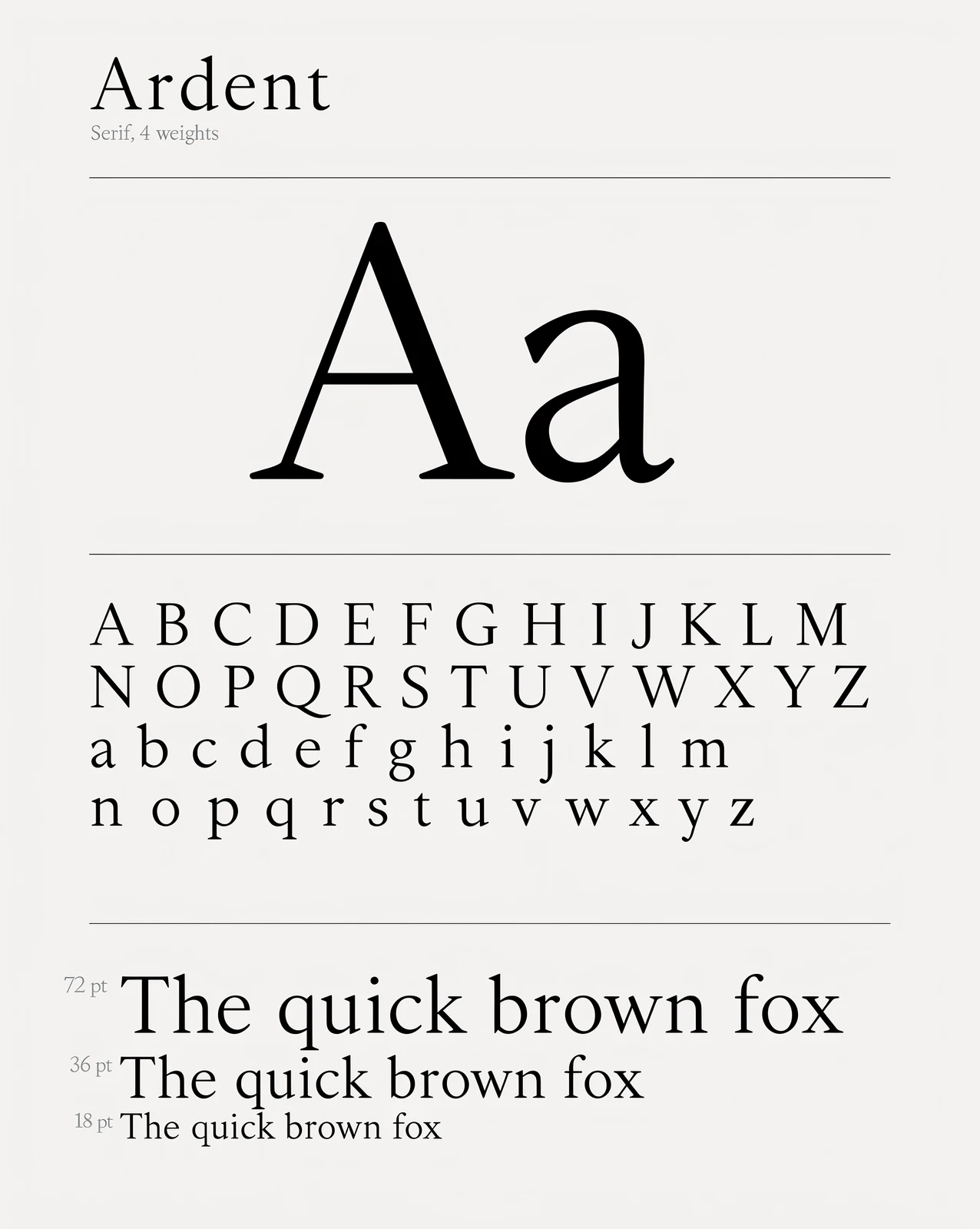
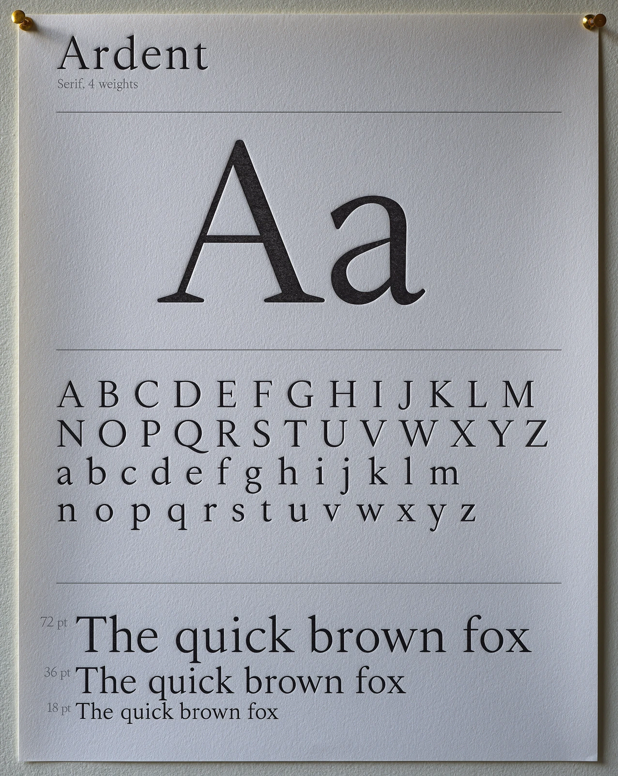
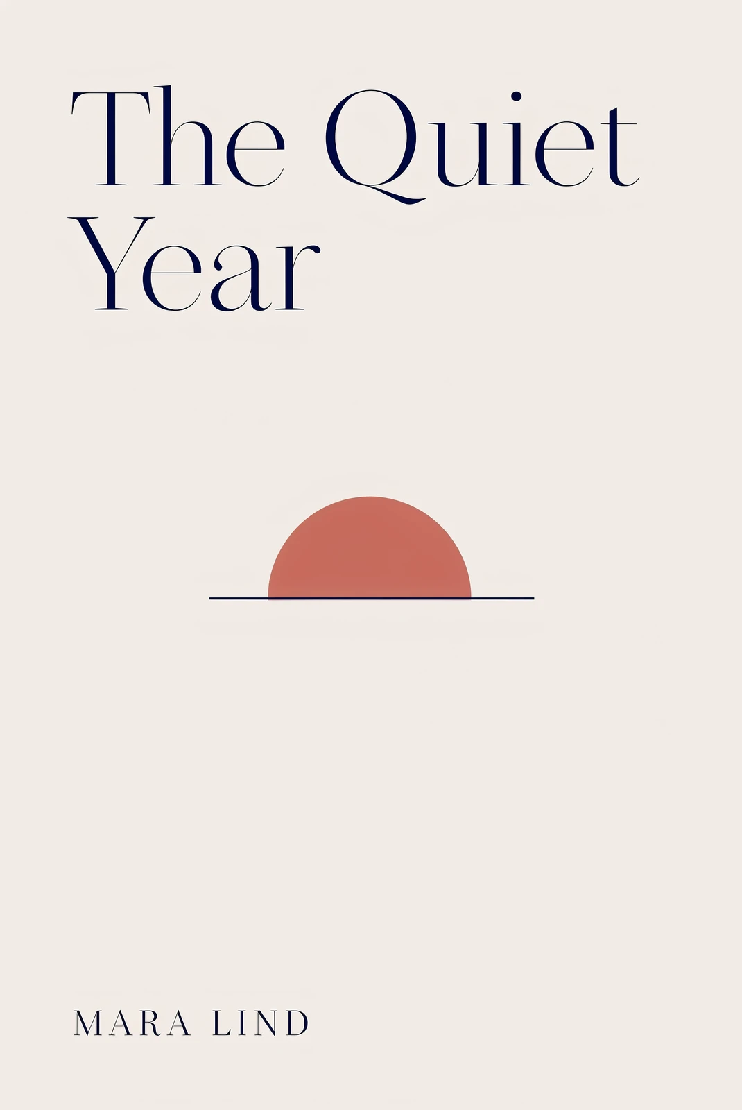

Our instructions always quote every string the output must contain, so the reward can compare the expected text with the text the model actually renders. Without careful calibration, such a reward also teaches the model to make its text easier to read at the cost of properties the edit should have.
Building the text plan. In image-to-image generation, the expected text depends on both the references and the instruction. For example, a replaced line has to disappear and every line the instruction does not mention has to survive. Before training, a planner agent therefore reads the instruction, the reference images and a blind read of each reference, and writes a text plan with three parts (Figure 20).
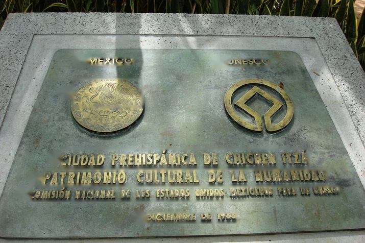
- MEXICO must survive
- UNESCO must survive
- ESTADOS UNIDOS MEXICANOS must survive
-
CIUDAD PREHISPÁNICA DE CHICHEN ITZÁCIUDAD PREHISPÁNICA Y PARQUE DE PALENQUE replaced - PATRIMONIO CULTURAL DE LA HUMANIDAD must survive
- COMISIÓN NACIONAL DE LOS ESTADOS UNIDOS MEXICANOS PARA LA UNESCO must survive
-
DICIEMBRE DE 1988DICIEMBRE DE 1987 replaced
On the bronze plaque, the raised brass lettering that read "CIUDAD PREHISPÁNICA DE CHICHEN ITZÁ" is replaced with "CIUDAD PREHISPÁNICA Y PARQUE DE PALENQUE", and the date line at the bottom that read "DICIEMBRE DE 1988" is changed to "DICIEMBRE DE 1987", matching the raised relief of the surrounding lettering. All other elements remain exactly as in the image.
Figure 20: A text plan from the RL pool, written once from the instruction and the blind read of the reference.
Verifying text accurately. To verify whether a model has rendered text correctly, we can use models trained specifically for optical character recognition (OCR), or VLMs. Traditional OCR (e.g., PaddleOCR [19]) and VLMs fail in opposite ways. Traditional OCR models are trained mostly on clean documents and are reliable for cases like graphic design and user interfaces that resemble text from typical document scans, but struggle with large typefaces, stylized fonts, in-the-wild text, and logos. We therefore use a VLM as our text reader, since it reads text more reliably under diverse conditions.
We ablated different methods of VLM-based OCR and found they perform best in a blind setting. Trying to include the editing instruction or reference images in the VLM’s input often causes it to autocorrect errors. For example, shown the word “eleghaant”, the VLM would read it as “elephant”.
Scoring against the plan. The harness then matches each string that must show to the rollout’s blind read. Similarity scores below 0.5 receive no credit, while exact matches receive full credit. A string that must not show has to be gone from where it stood, and every line that must survive has to be found again, with each line scored on its own. The three component scores are then combined into one text reward.
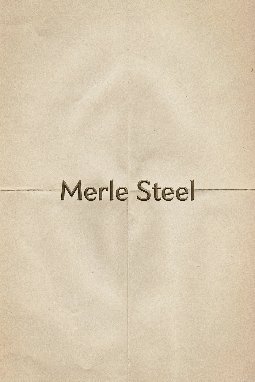
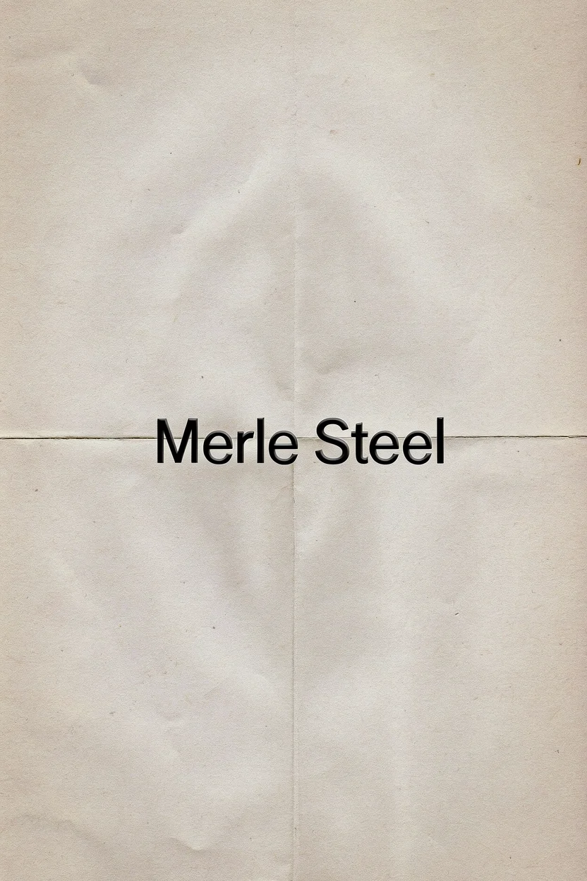
Reward hacking. Despite their strong generalization, VLMs are not fully accurate. Small or stylized text can be misread even when it is rendered correctly, so an easy way to hack the text reward is to make text bolder, bigger, higher in contrast and plainer in style. In one of our runs, the model learned exactly this while its text reward kept rising (Figure 21, top). To mitigate this behavior, we added a size penalty similar to the length penalty in LLM RL, which caused a different failure mode, where the model learned to shrink text (Figure 21, bottom).
heavier, generic type
Write "Merle Steel" on the paper.
smaller type
Add the text "Smooth moments, bold flavor." in an appropriate position.
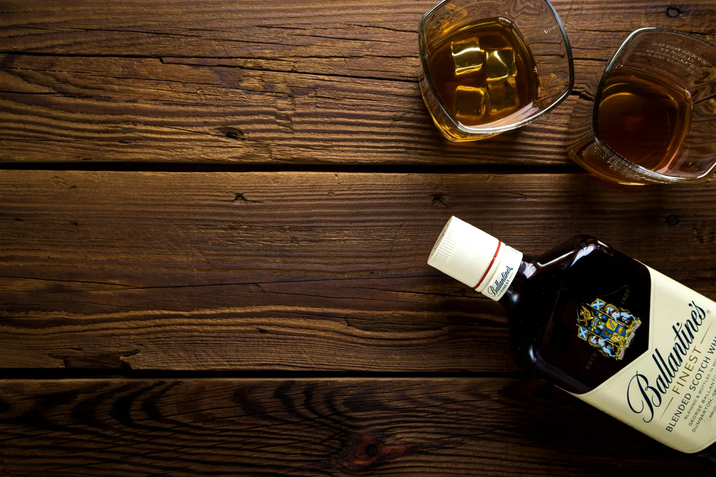
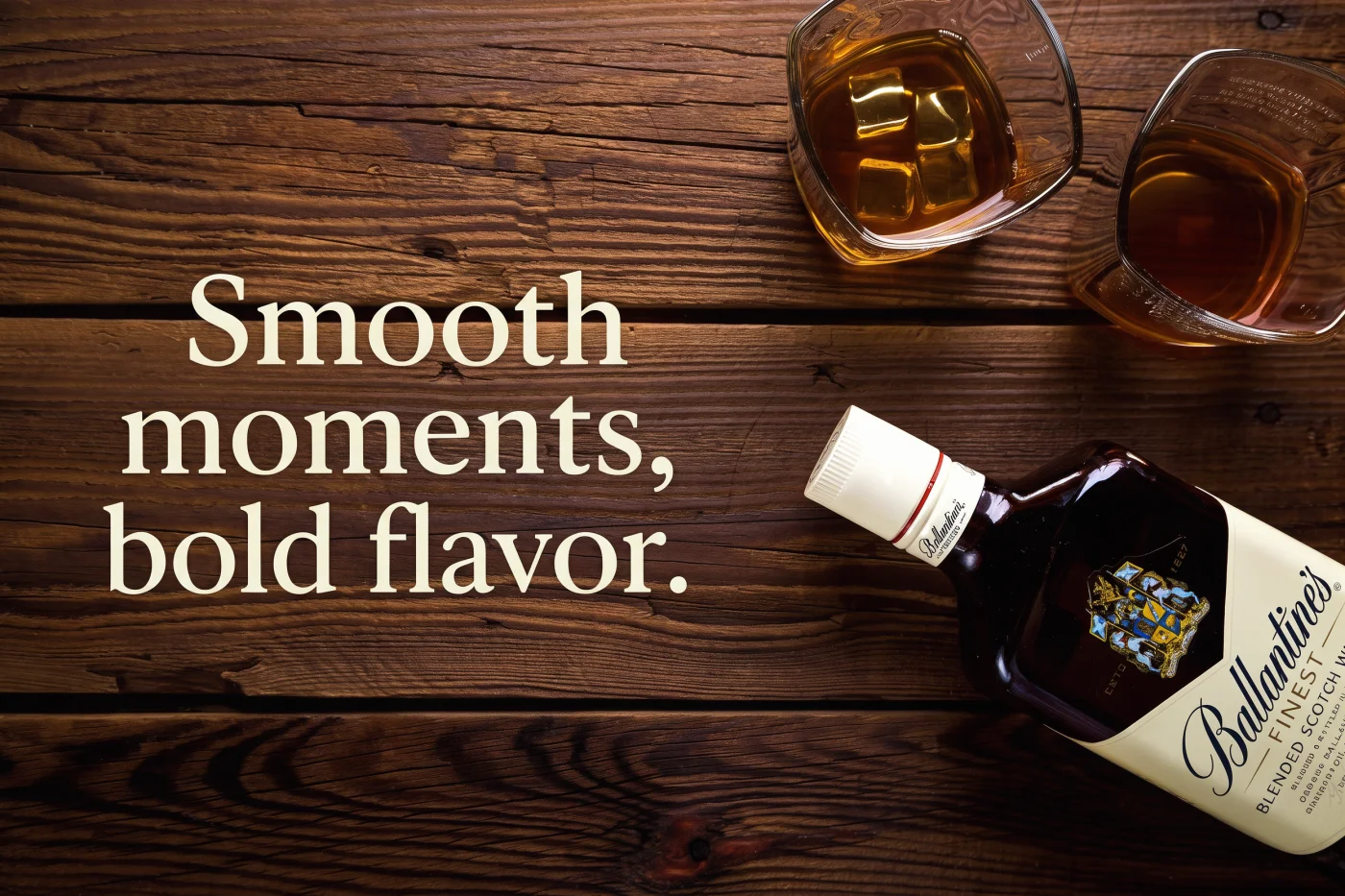
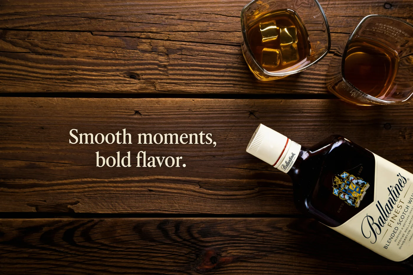
Public text-editing benchmark items, same prompt and seed, before and after RL with earlier versions of our text reward.
Figure 21: Two shortcuts that earlier text rewards reinforced, with the same prompt and seed before and after RL.
The final fix has two parts.
- A typography judge scores only the text the edit added or changed and evaluates whether the edited text fits the overall design of the image.
- A size constraint measures every rendered line against a fixed anchor, never against the rest of the group. A second term penalizes a drift toward larger or smaller text that is shared across the whole batch.
With these fixes in place, the share of changed text flagged as heavier than the design fell from 28% to about 10% with no sign of size drift over the first 60 steps of RL training.
Region rewards
For local edits, the most important requirement is usually implicit: the image should remain unchanged outside of the edited region.
Inputs with this requirement are given a region plan by the reward harness during dataset preprocessing, which defines a bounding box where the edit should take place. A correct local edit often changes surrounding areas: an object added to a scene may cast a shadow, so we calibrate the planner to account for such side effects.
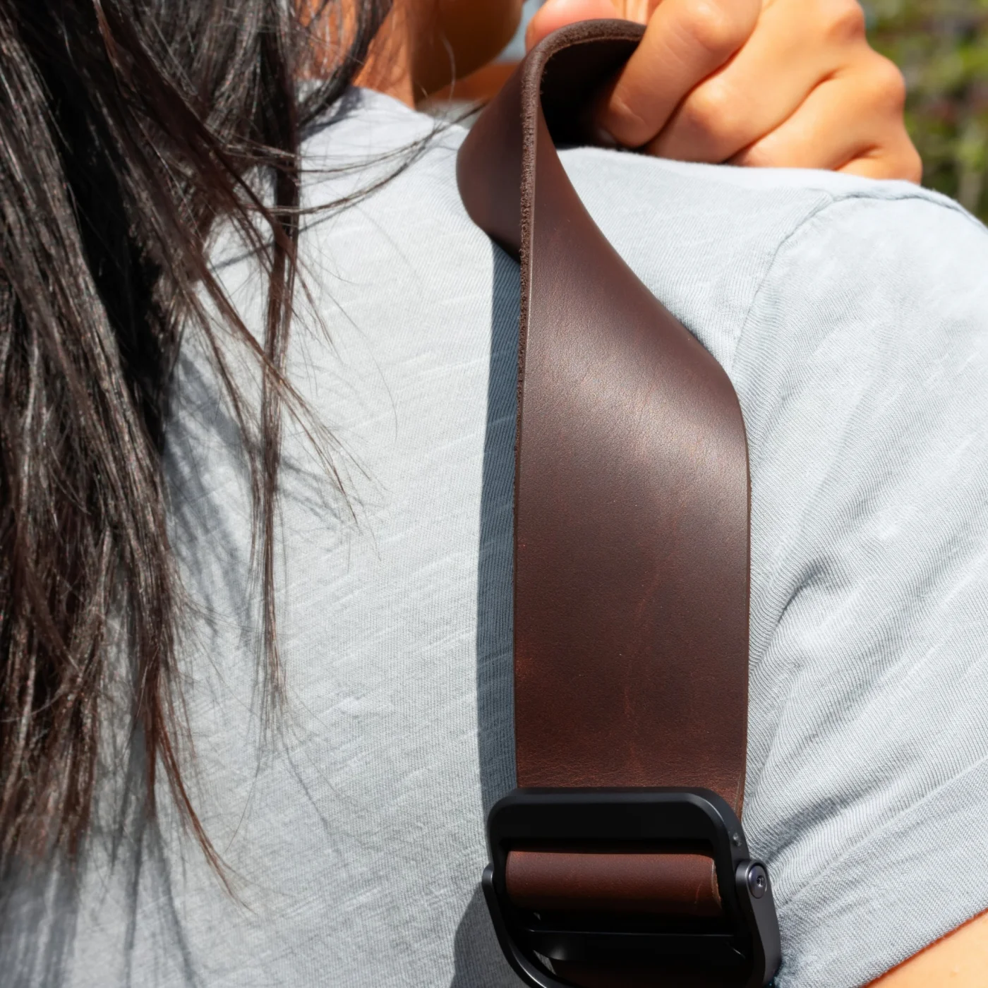
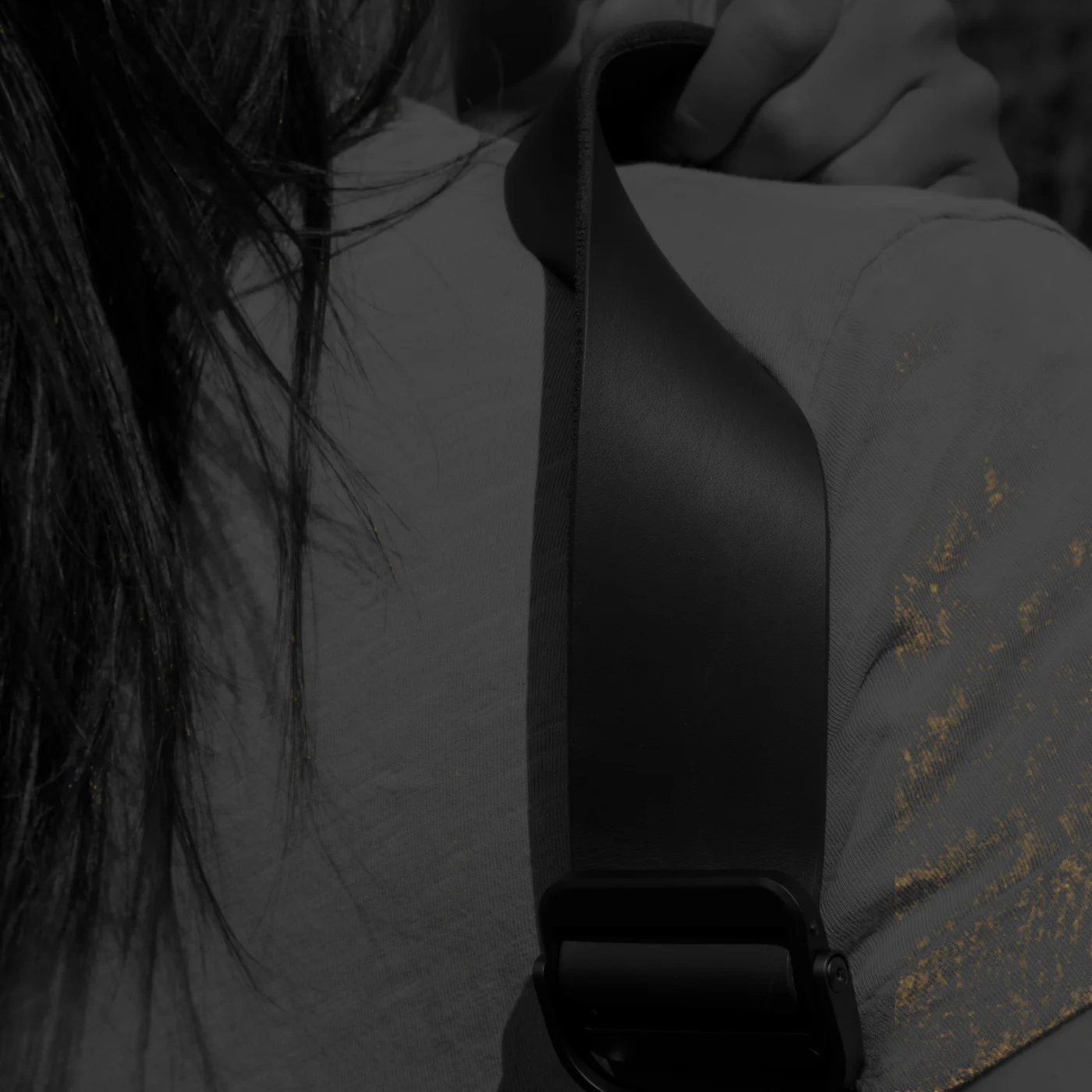
During training, a pixel-level reward on rollouts verifies that the image remains unchanged outside of the planned edit region (Figure 22).
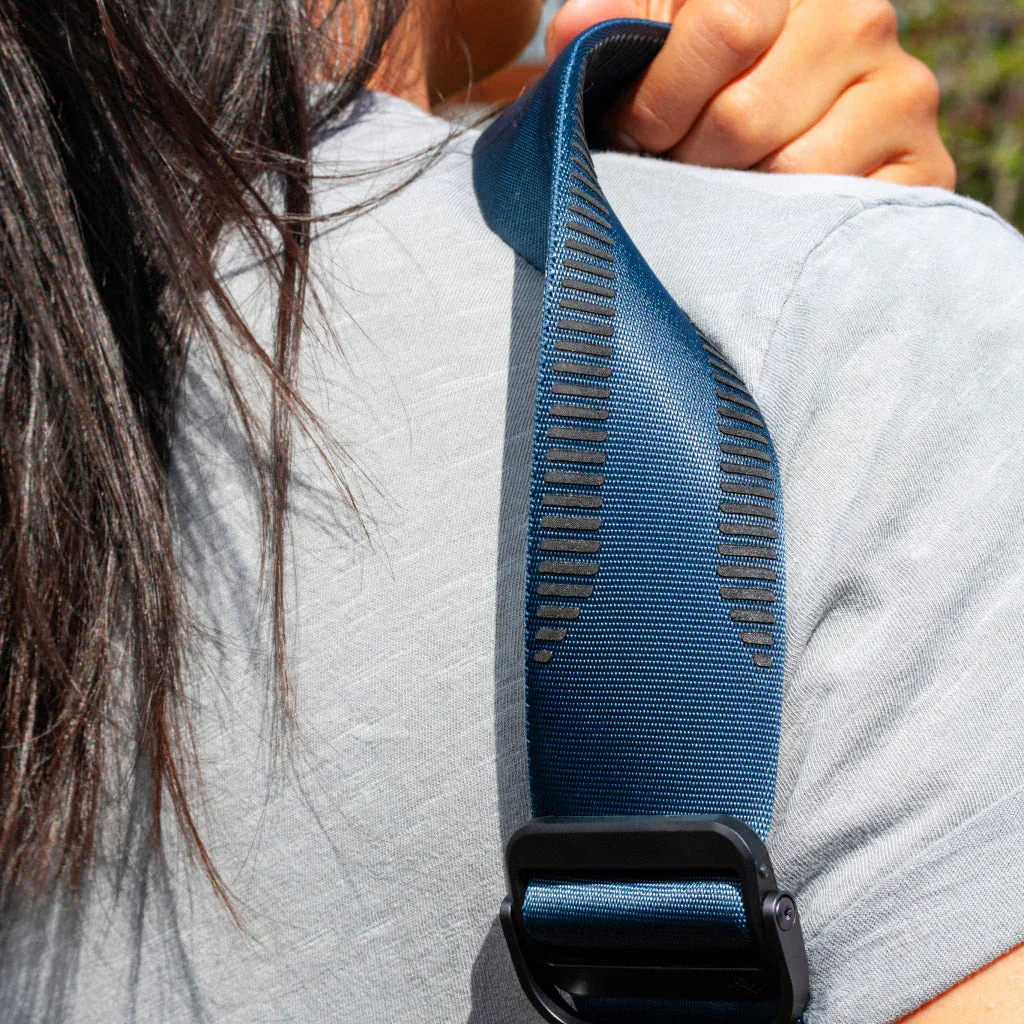
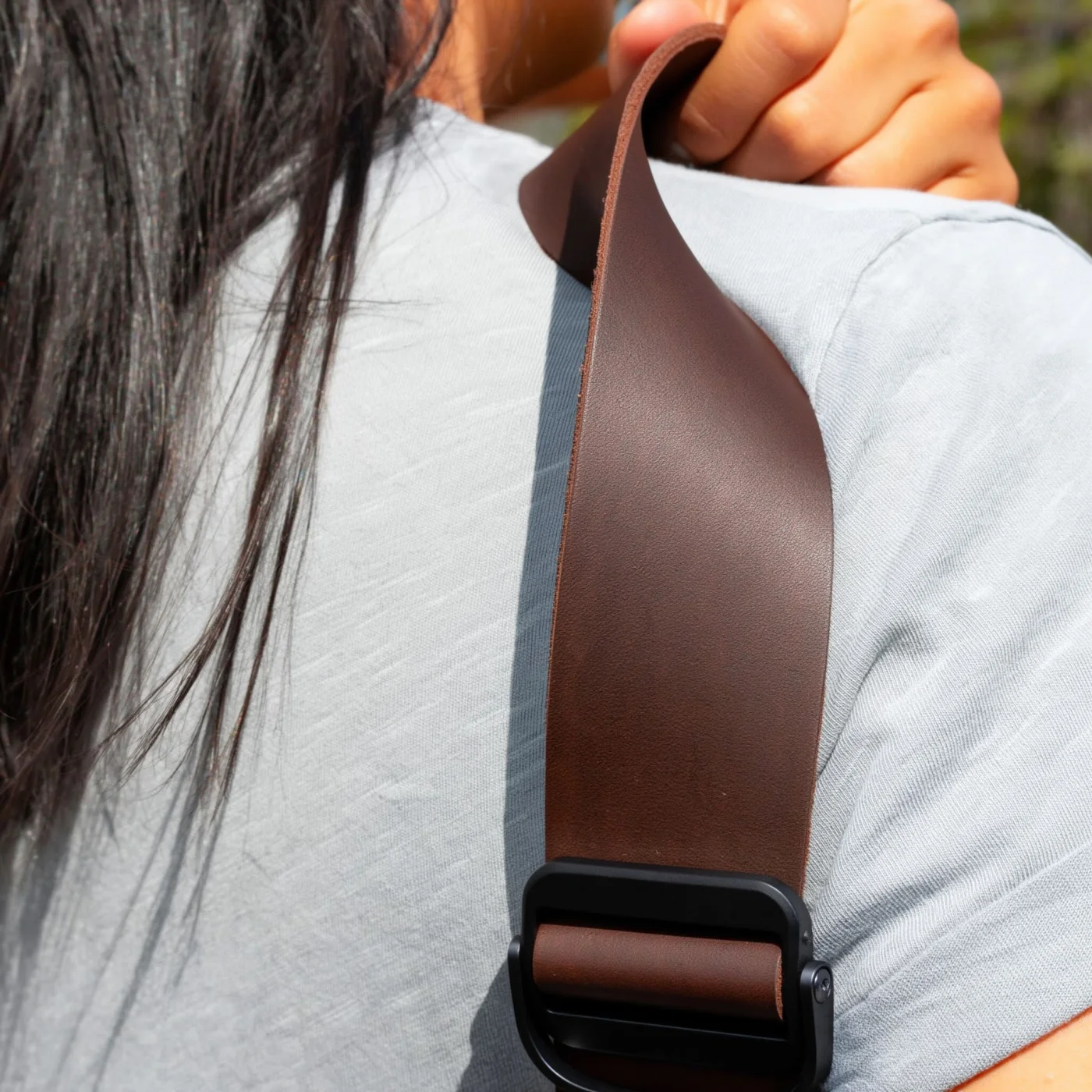
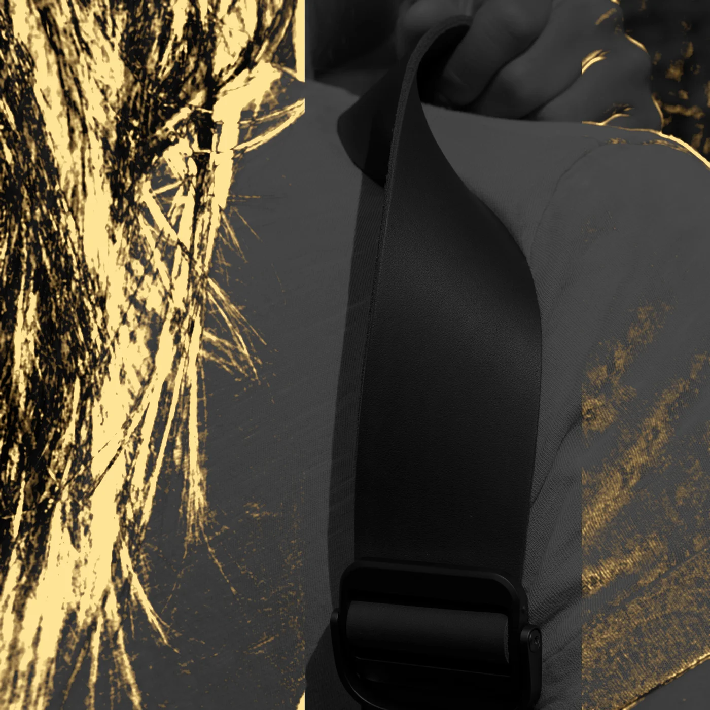
Replace the blue nylon strap with a dark brown leather strap. Keep the hand, hair, shirt and framing exactly as they are.
rollout A kept everything outside the strap
- region reward
- 0.88
- preference judge
- 0.50
- rubric judge
- 0.44
- advantage
- −0.01
rollout B redrew the hair, outside the region
- region reward
- 0.27
- preference judge
- 0.25
- rubric judge
- 0.50
- advantage
- −0.35
Figure 22: The region reward catches three rollouts that redrew the hair outside the planned region.
In isolation, a regional pixel preservation reward leads to reward hacking, like copying the entire reference image unchanged. Therefore, the region reward is always combined with other rewards like preference and rubric judges, which would penalize an unchanged copy and ensure its advantage is lower than that of a rollout that actually performed the edit.
Combining rewards
Once we have computed all of the rewards for the rollouts in a group, we combine them before converting them into advantages. These rewards are on different scales, so following Group reward-Decoupled Normalization Policy Optimization (GDPO) [20], we normalize each reward within its group before combining them so that no reward dominates by scale.
We also measure how noisy each reward is by scoring the same rollouts twice, and after normalizing we weight that reward’s advantages in each group by how much its variance within the group exceeds this noise. When a reward’s variance within a group is no larger than its own noise, that reward adds nothing to the group’s advantages, so a judge’s coin flip between two equally good edits does not become a full-size advantage.
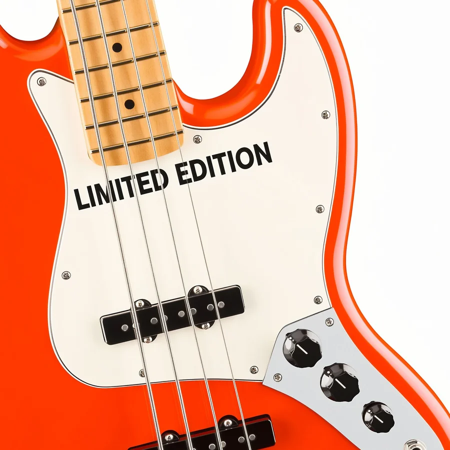
Figure 23 shows one real group from our RL training, where the instruction asks for “LIMITED EDITION” in bold black capitals on the white pickguard, right above the neck pickup. The four edits in the top row are the most successful and receive the highest advantages. On the bottom row, the rollouts fail in different ways. Left to right:
- the text is rendered too large
- “EDITION” is garbled and illegible
- the plate at the bottom right turned black
- the text is too large and misspelled
This group shows how our multi-reward design makes our RL robust to noise and error in individual rewards. No single reward detects all of these failure cases. The text reader scored the garbled edit as fully correct, and the preference judge scored the oversized edit above most of the group, yet the combined rewards rank all four failures below the clean edits.
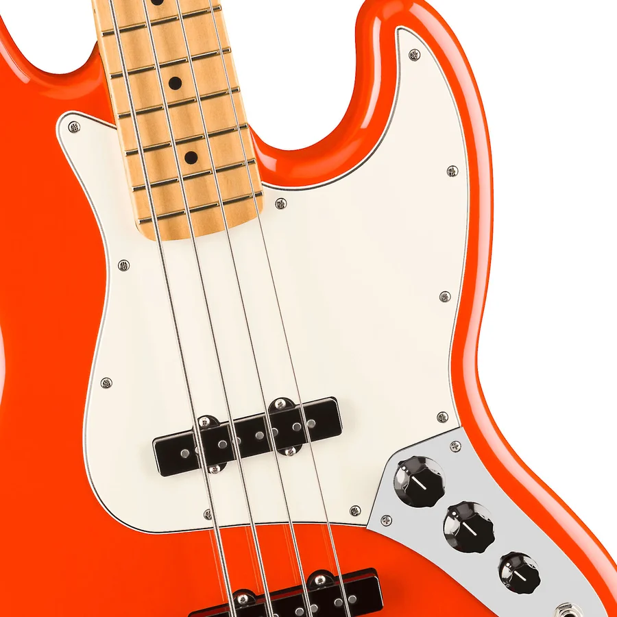
Please add the text 'LIMITED EDITION' printed in bold black capital letters onto the white pickguard, right above the neck pickup.
shown here the other eight
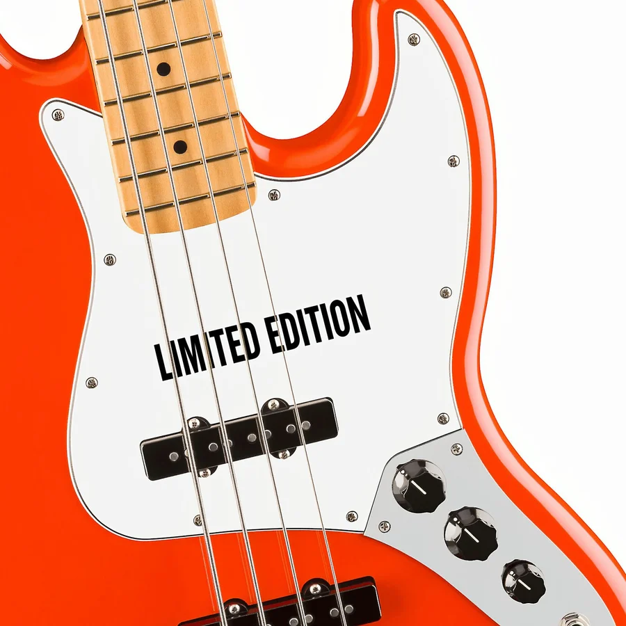
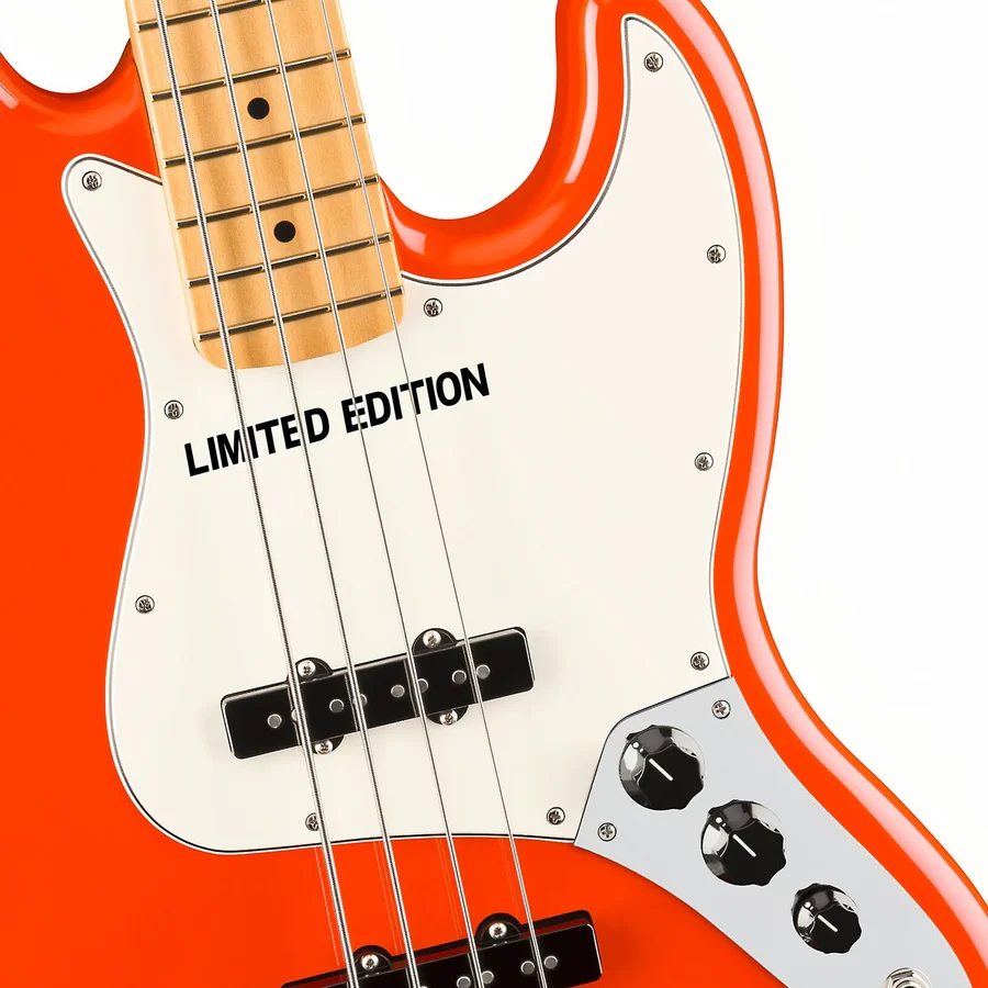
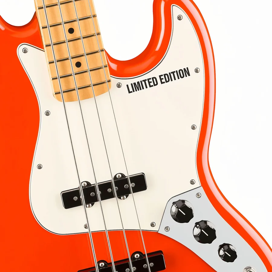
All four: spelled right, black capitals above the pickup, rest of image unchanged
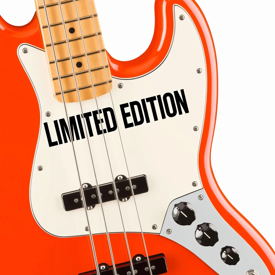
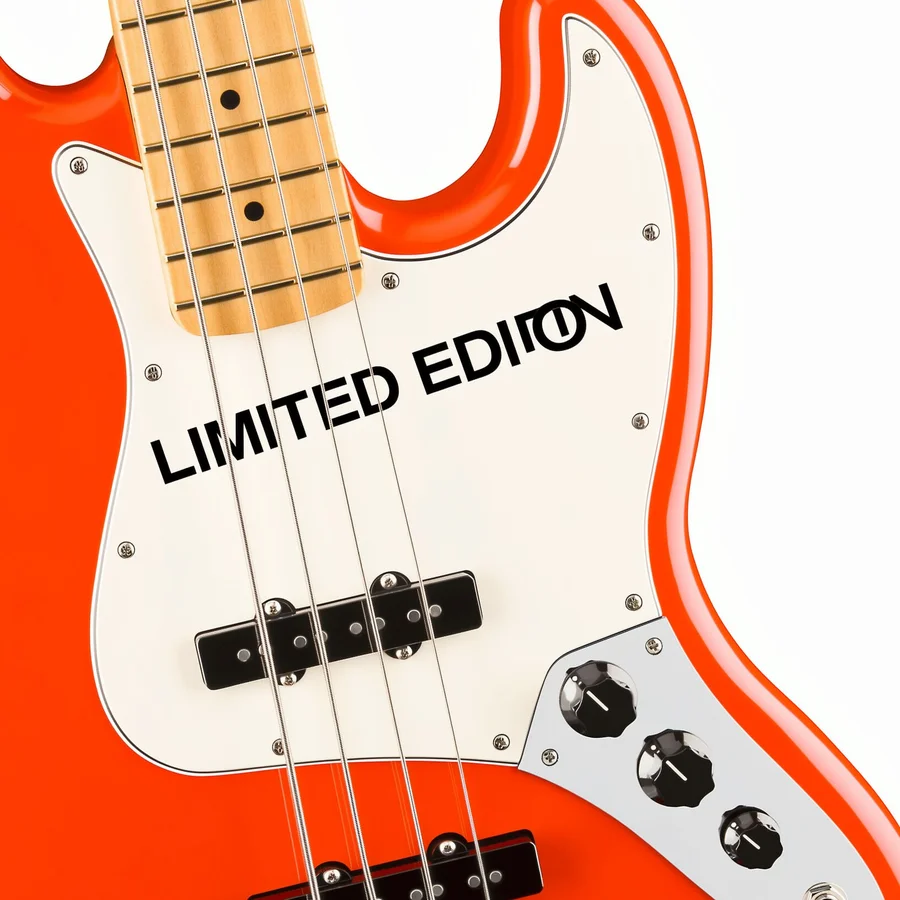
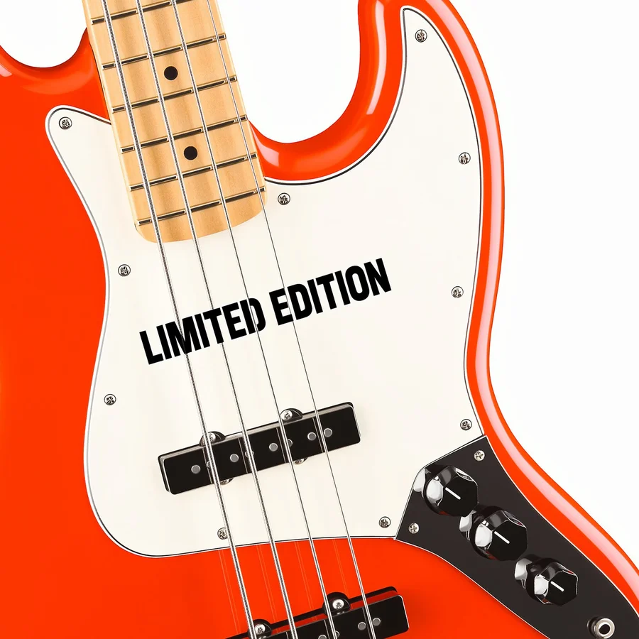
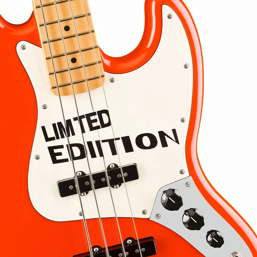
Figure 23: One real training group, sorted by advantage. Grey lines name the rewards that caught each failure.
Keeping the group diverse
Group-relative RL can only learn from differences between the rollouts of a group. In LLM RL this variation comes almost for free, because temperature sampling sends each rollout down a different chain of reasoning, and pass@k [21] climbs quickly with k. Diffusion rollouts vary much less, especially when they are sampled with a deterministic ordinary differential equation (ODE) solver, where the only randomness left is the initial noise. Classifier-free guidance [22] then pulls every noise sample toward the same mode of the conditional distribution, so sixteen seeds of one instruction tend to provide very little reward variance between the rollouts.
We measured this on 97 hard inputs where our pre-RL model struggles. Generating a single output per task, the model does not successfully complete a single one. With 16 generations per task, varying the initial noise between attempts, only 7 of the 97 tasks have at least one correct generation. Moreover, the failed samples nearly always repeat the same mistake. Varying the guidance scale does not help either.
Paraphrasing the instruction, on the other hand, does what changing the seed cannot. We define a paraphrase as a rewrite of the original instruction. The paraphrase preserves the intent and every quoted string of the instruction, changing only the wording. With ten attempts for each of the 97 hard inputs, using different paraphrases for each attempt solves almost twice as many cases as only varying the seed.
We therefore make sure every group provides training signal in two ways.
- Filtering RL input data. We apply offline filtering to make sure a group generated with our pre-RL checkpoint has sufficient reward variance. Similar to dynamic sampling in DAPO [23], we also clean the pool online during training, retiring an input once its rewards saturate and replacing it with a new one.
- Instruction paraphrasing. Half of the rollouts in each group use a constrained paraphrase of the input instruction that the augmentation agent writes offline. A judge rejects any paraphrase that contradicts the rubric generated for the original instruction. Every rollout is still scored and trained against the original instruction. Thus, the paraphrase changes where the model explores but not what it is rewarded for, and the paraphrased rollouts stay close to on-policy.
What RL changed
RL made Krea 3 fail less often. We saw substantial improvements in text rendering and on tasks that need reasoning. In our latest RL run, the rewards for text, typography and unedited pixels rise over the first 60 steps on inputs the model has not trained on (Figure 24, left). On held-out sets, the RL stage of Krea 3 cut text errors on public text-editing benchmarks by about a quarter. On CPI-Bench [24], scored by its own judge, which we never trained against, we reduced the rate of flawed generations by 17% and by 27% in its “intelligent” category, where the model failed most often before RL (Figure 24, right).
Figure 24: Rewards over the first 60 RL steps (left), and held-out text errors and flawed CPI-Bench edits before and after RL (right).
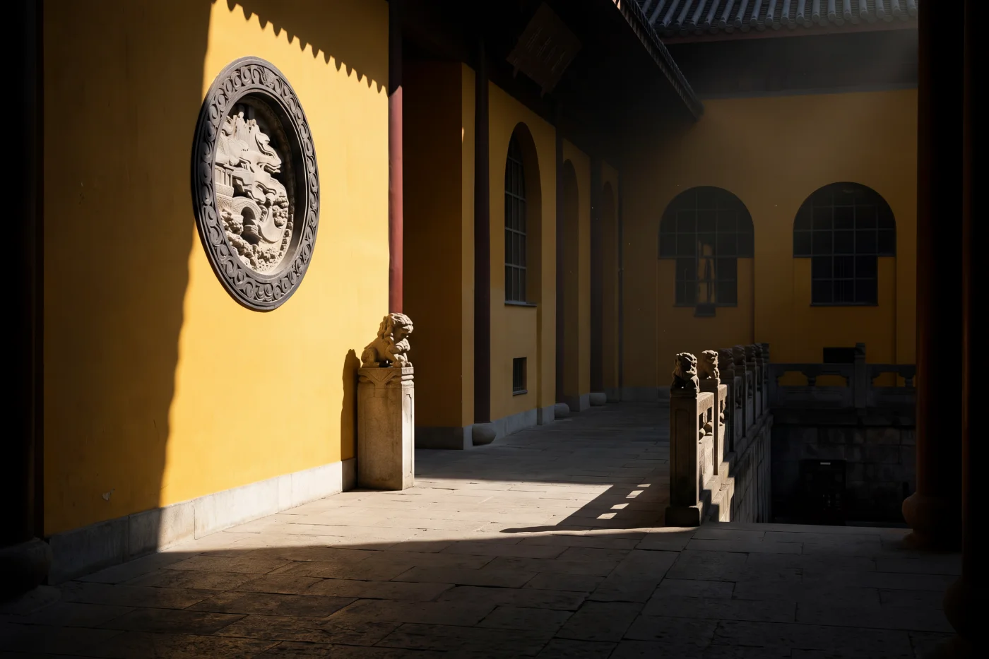
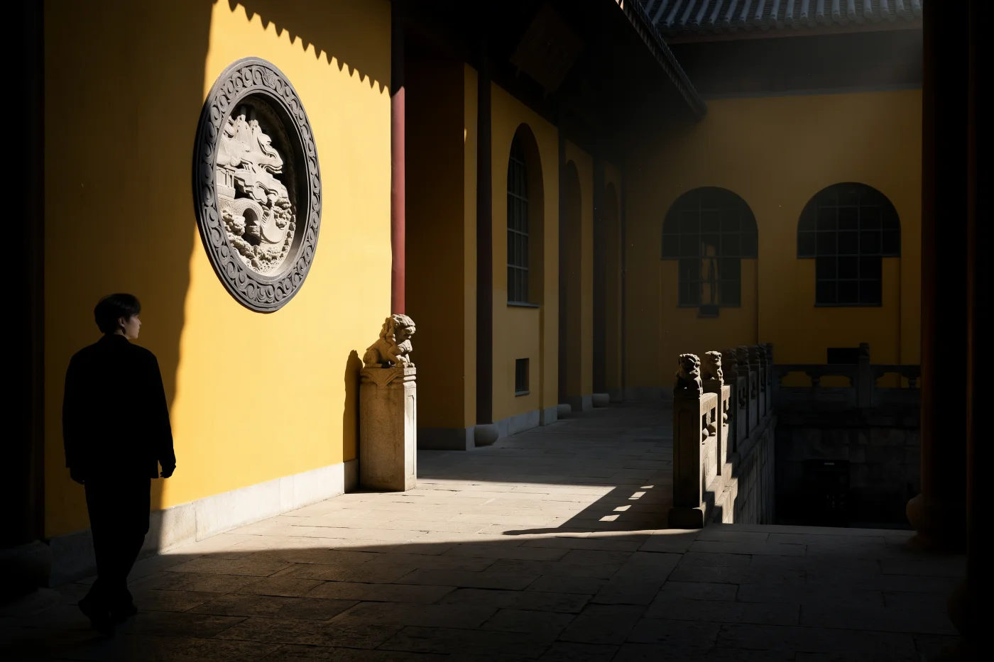
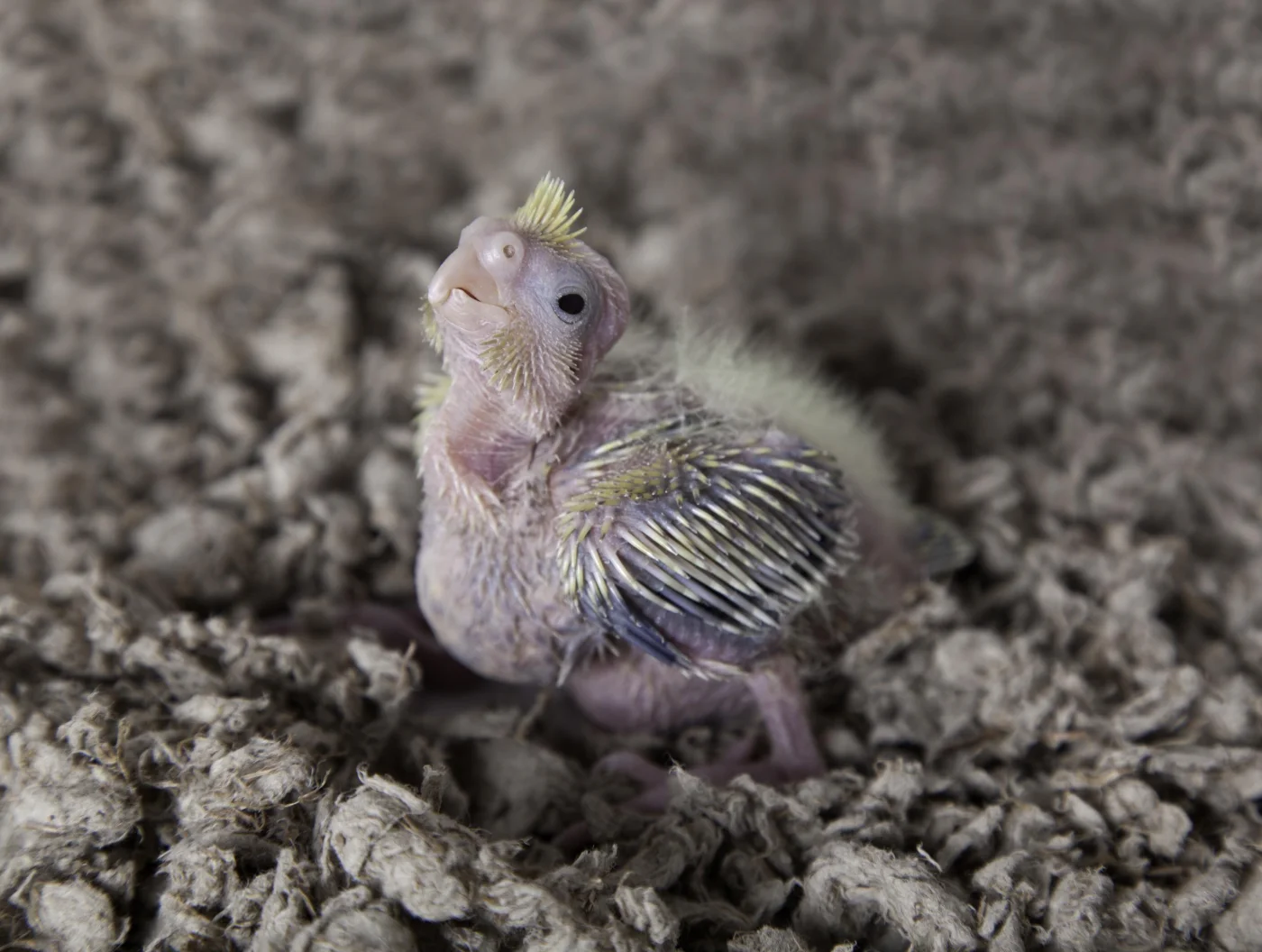
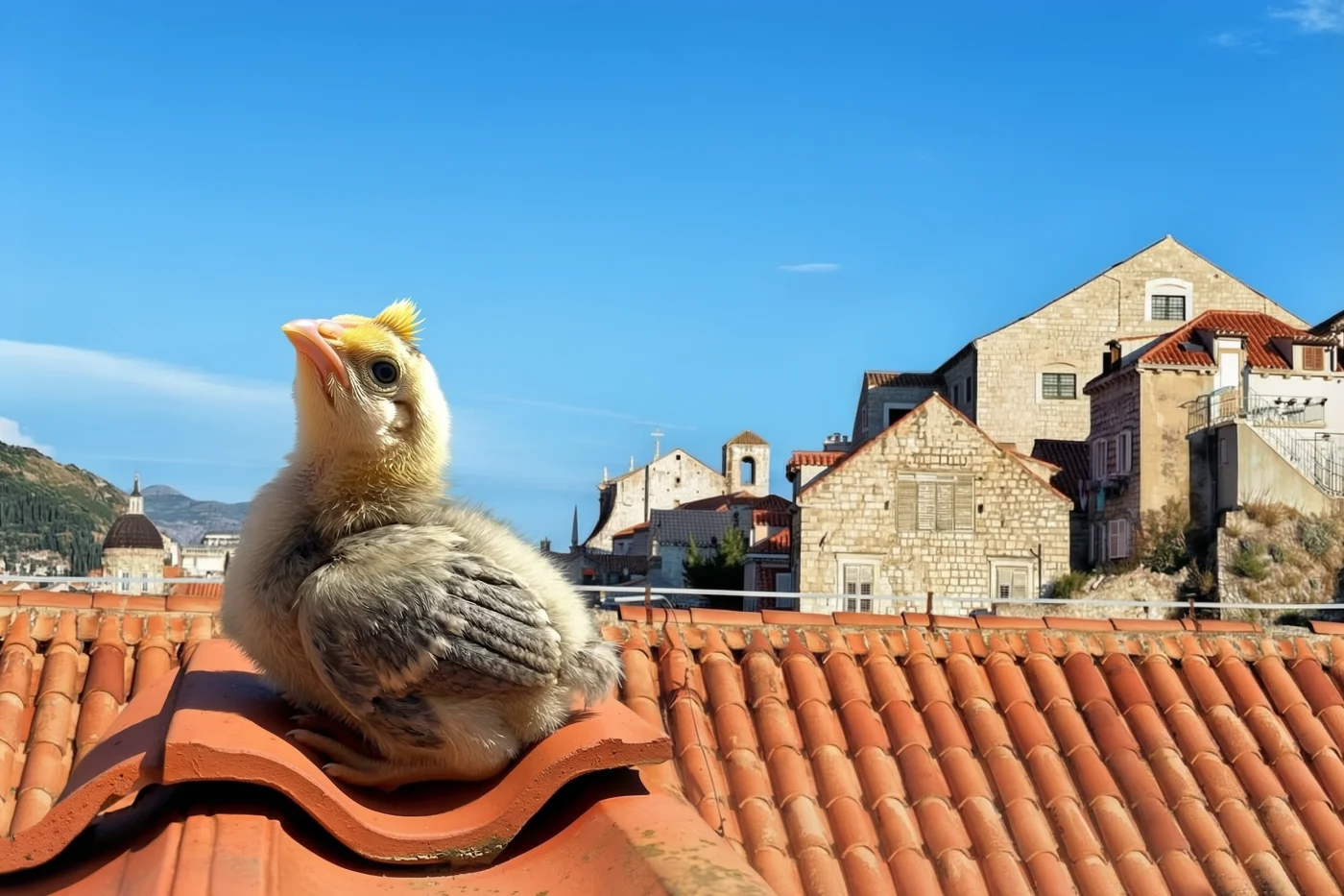
Figure 25 shows held-out edits that RL fixed. Before RL, the model left half of a poster’s headline in Chinese and garbled the rest, removed a man along with the woman it was asked to remove, pasted a giant generic chick in place of the one in the reference, and turned a saucepan’s handle copper when only its leaf ornaments were meant to change. After RL, each edit follows the instruction more precisely and doesn’t make unintended changes.
translate a poster
Translate the text into English.
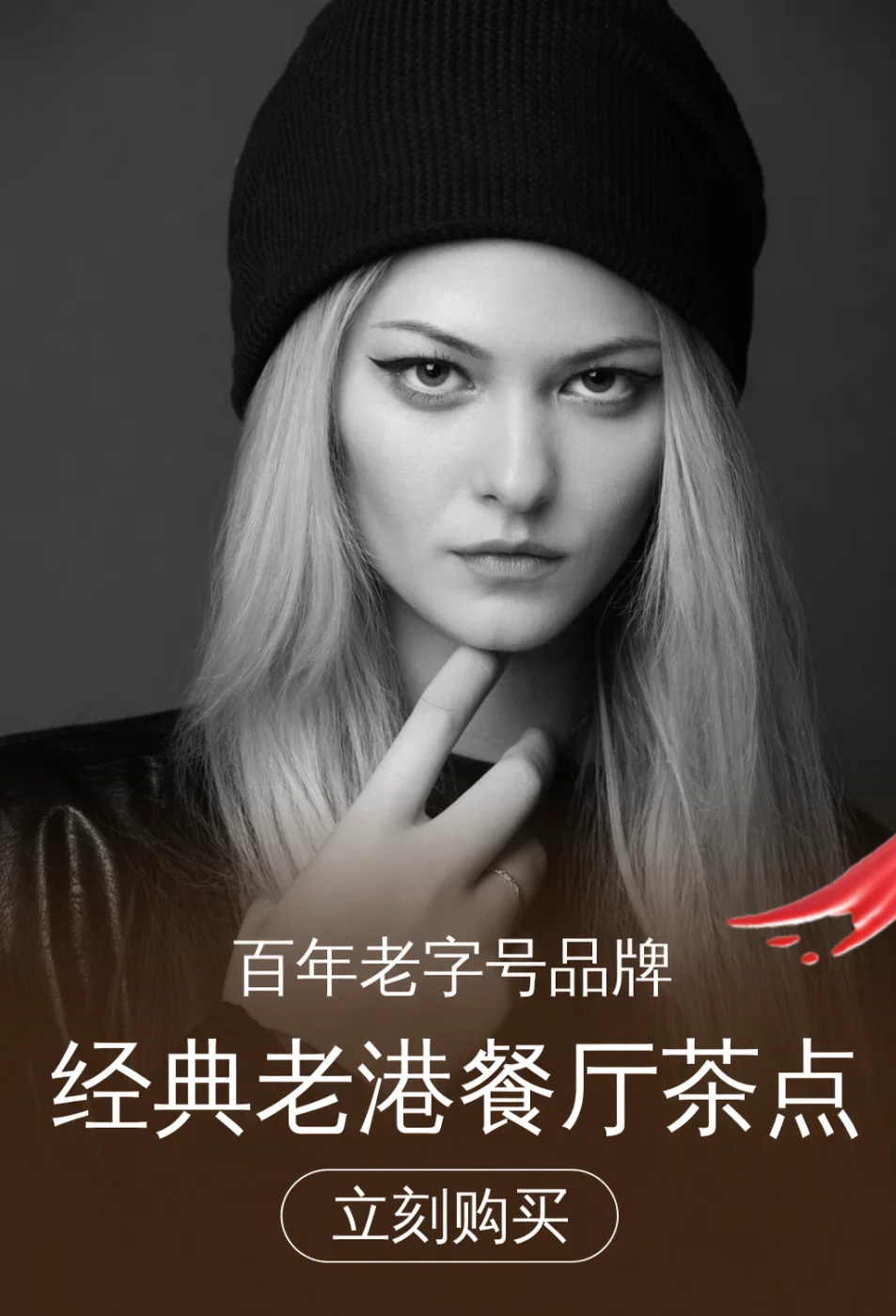
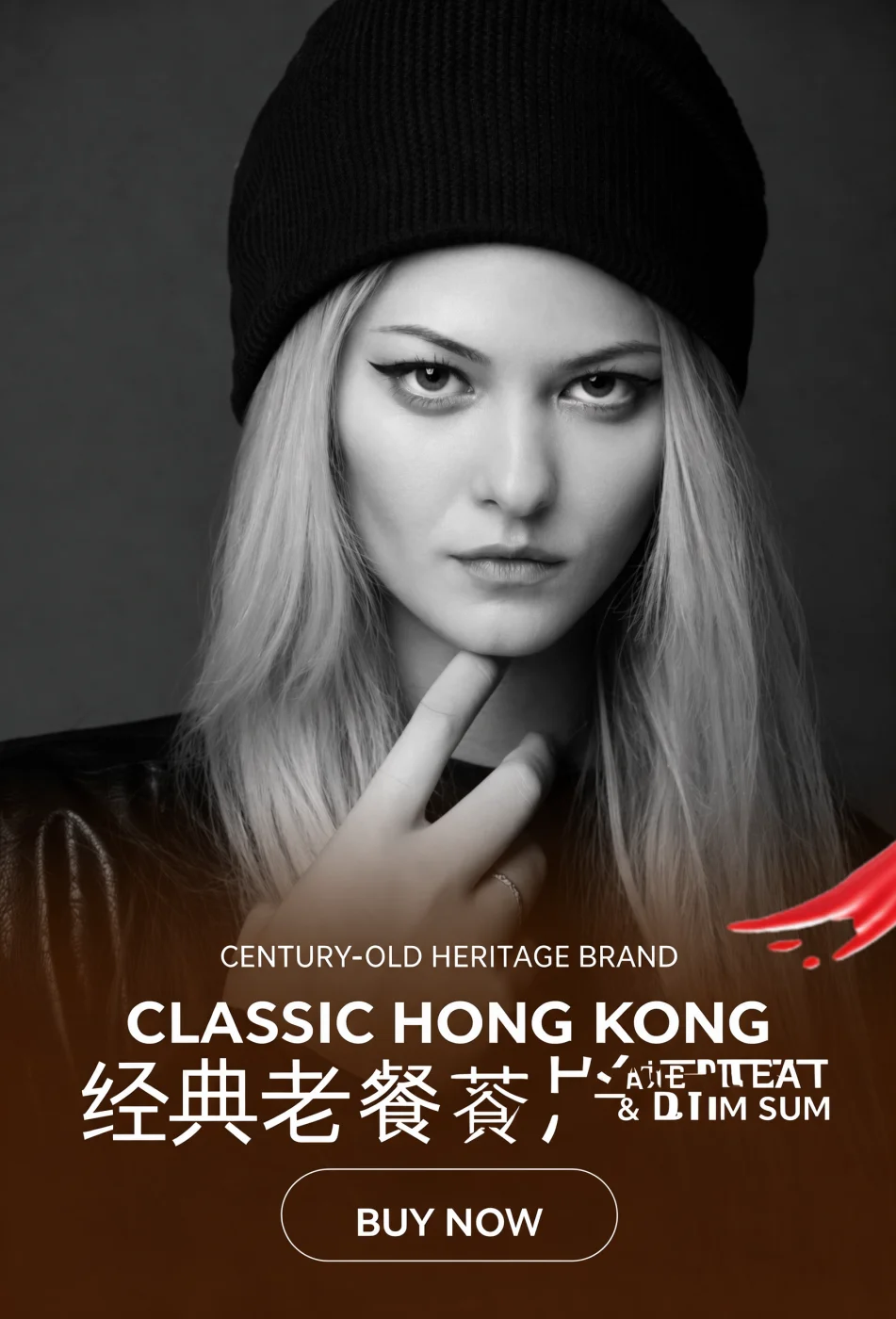
half the headline left in Chinese, the rest garbled
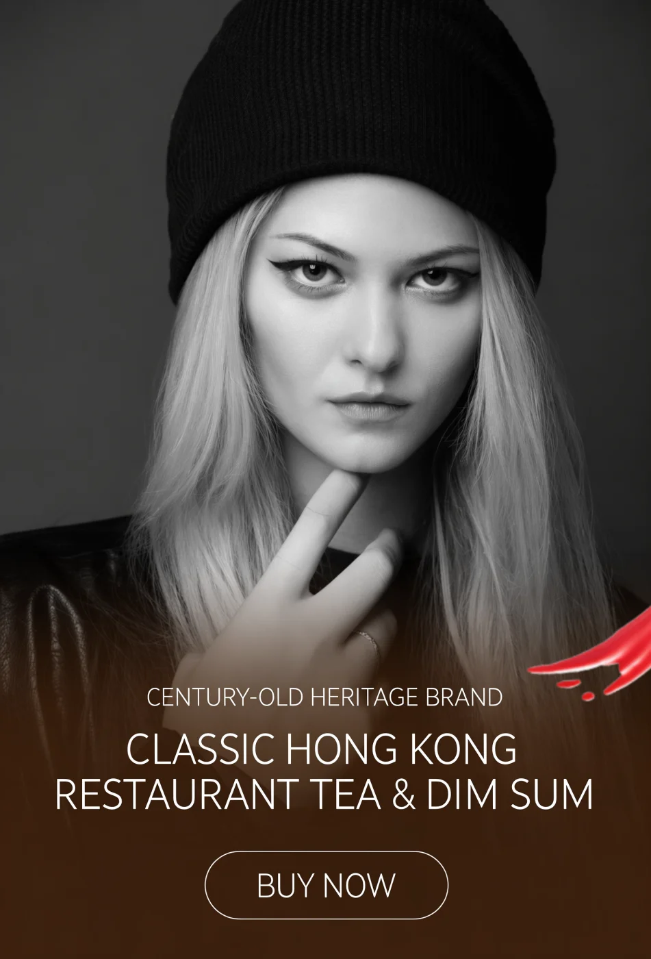
the whole poster in English, every line legible
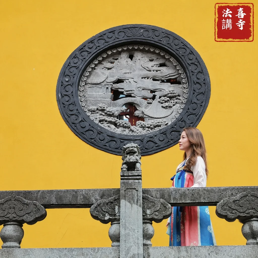
remove the person the reference shows
Refer to image 2 and remove the same woman from image 1.
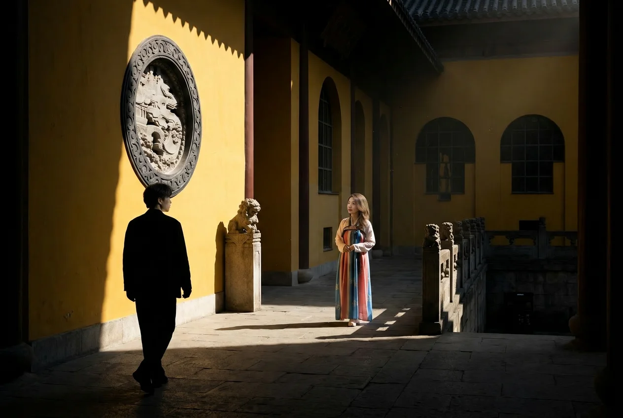
removed the man as well
only the woman is gone
the chick from the reference, at its size
Place a yellow-gray fluffy chick looking up at the blue sky on the red tile roof.

a generic chick, giant, on a broken tile

the chick from image 1, at a plausible size
only the part that was named
Change the silver leaf handle ornaments to polished copper finish.
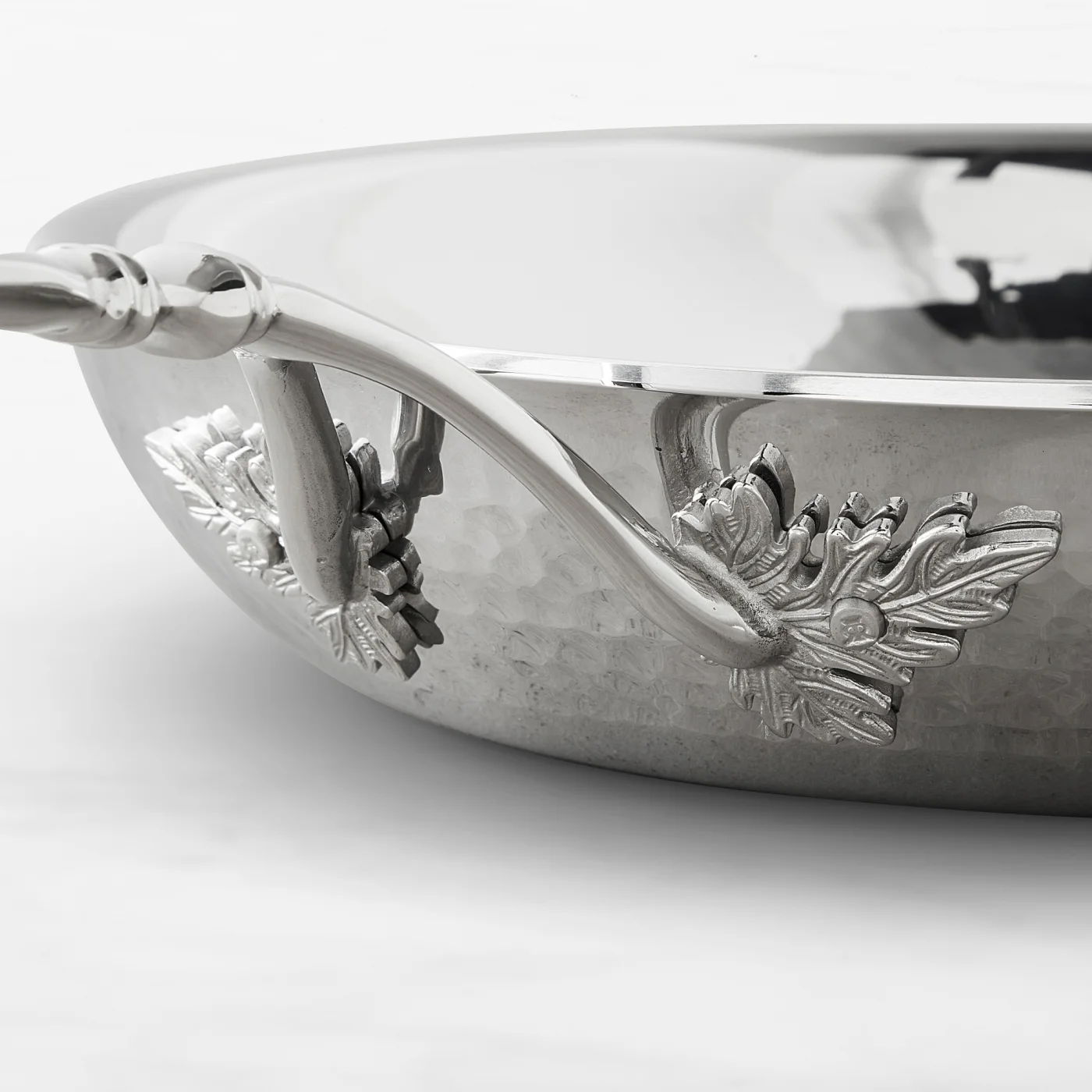
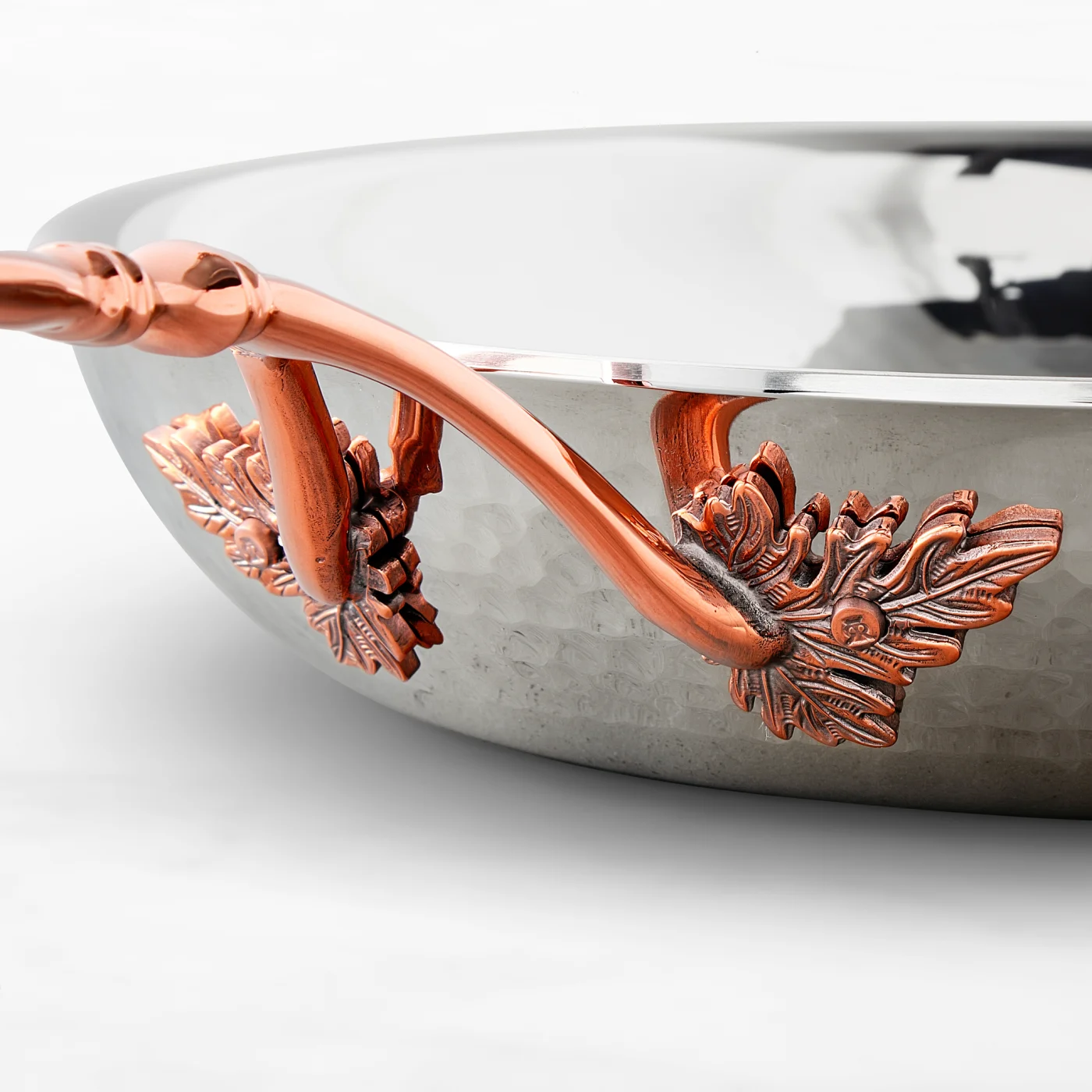
the handle bar turned copper too
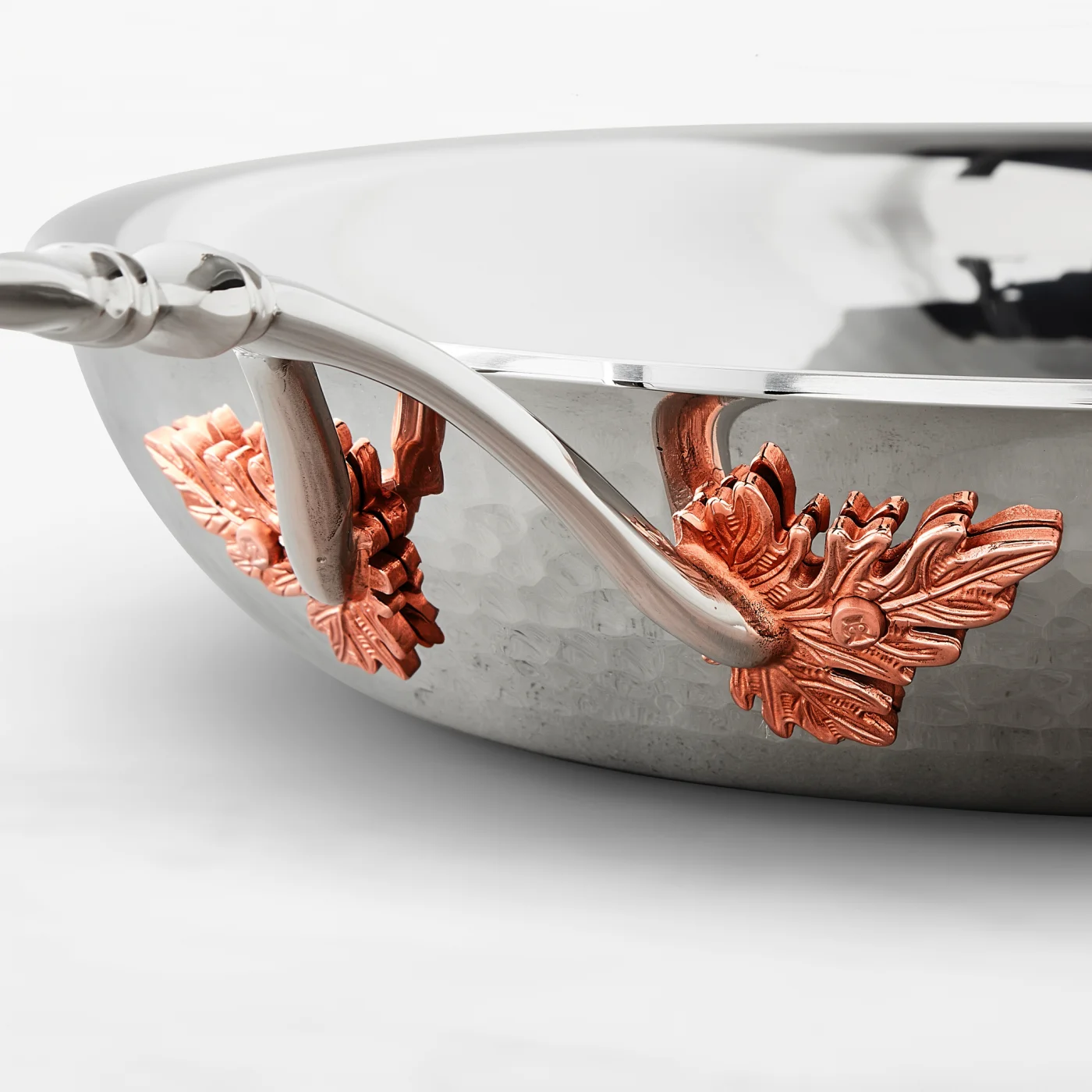
only the leaf ornaments change
Figure 25: Held-out edits before and after the RL stage of Krea 3.
Preference optimization
After RL, we apply a lightweight preference optimization stage, which aligns the model with human preference on qualities that our judges cannot check reliably, such as fine texture and identity. We use DPO [25, 26] on preferences from in-house labelers. The standard DPO loss allows the model to satisfy the training objective merely by unlearning the loser distribution rather than learning the distribution of winning images, so we anchor the loss on the preferred images following ThermoDPO [27].
In our experiments, DPO worked best on global properties of the output distribution: high-frequency texture, color shift, and brightness balance all improve reliably. Small text rendering, by contrast, improves less under DPO and is more prone to preference hacking, even with careful hyperparameter tuning.
DPO is also excellent for complex identity preservation. Humans are very good at detecting subtle shifts in facial identity across images, while VLM judges miss fine identity inconsistencies and face embedding models are not robust to strong changes in pose, expression, lighting, or occlusion. Human preference is therefore the more reliable signal for these cases.
Limitations
- Small text. As with many frontier models, extremely dense small-text rendering is still imperfect, and it is a clear target for future work.
- Identity and character consistency. Like the rest of the field, Krea 3 is not perfect at preserving identity across edits. Many frontier models still resort to directly copying the reference image to preserve identity and character consistency. We aim to use LoRAs as our main tool to close this gap for specific characters and products.
Discussion and future work
Efficient architectures
Training at higher resolution was one of the most effective changes this cycle, and 2K or even 4K generation clearly helps resolve fine details such as small text. But image token counts grow fast with resolution. For the next iteration, we plan to explore architectures that scale image tokens more efficiently.
Toward realtime editing
Krea 3 is fast, but not yet real time. The fastest configuration today completes an edit in about 4 to 5 seconds. We will keep doubling down on speed, since every reduction in latency changes how people work with an editing model.
Editing interfaces
Because editing accepts such a flexible input format, we want the model to natively understand more ways of expressing an edit, including visual annotations and instructions written on the image, and we will keep building data pipelines for them.
Scaling
We believe that we have barely scratched the surface of scaling our methods across data, pretraining, and reinforcement learning. Our team is constantly exploring better pretraining recipes and efficient methods to scale our data and RL pipelines.
Conclusion
Krea 3 is built on the belief that once image-to-image intelligence is good enough for production, speed, cost, and personalization are the next frontier. Krea 3 combines high-quality editing with fast, cost-efficient serving, and can be personalized with custom data. We are continuing to push towards scale, efficiency, controllability, and realtime generation in our upcoming foundation models.
References
- Sangwu Lee et al. Krea 2 Technical Report. 2026. krea.ai/blog/krea-2-technical-report
- Diederik P. Kingma and Max Welling. Auto-Encoding Variational Bayes. ICLR 2014. arXiv:1312.6114
- William Peebles and Saining Xie. Scalable Diffusion Models with Transformers. ICCV 2023. arXiv:2212.09748
- Patrick Esser et al. Scaling Rectified Flow Transformers for High-Resolution Image Synthesis. ICML 2024. arXiv:2403.03206
- Jiaming Sun et al. LoFTR: Detector-Free Local Feature Matching with Transformers. CVPR 2021. arXiv:2104.00680
- David G. Lowe. Distinctive Image Features from Scale-Invariant Keypoints. IJCV 60(2), 2004. PDF
- Oriane Siméoni et al. DINOv3. 2025. arXiv:2508.10104
- Michael Tschannen et al. SigLIP 2: Multilingual Vision-Language Encoders with Improved Semantic Understanding, Localization, and Dense Features. 2025. arXiv:2502.14786
- Qwen Team. Qwen3.5: Towards Native Multimodal Agents. 2026. Model cards: Qwen3.5-9B, Qwen3.6-27B
- Lvmin Zhang et al. Adding Conditional Control to Text-to-Image Diffusion Models. ICCV 2023. arXiv:2302.05543
- Zhihong Shao et al. DeepSeekMath: Pushing the Limits of Mathematical Reasoning in Open Language Models. 2024. arXiv:2402.03300
- Kaiwen Zheng et al. DiffusionNFT: Online Diffusion Reinforcement with Forward Process. ICLR 2026. arXiv:2509.16117
- Anisha Gunjal et al. Rubrics as Rewards: Reinforcement Learning Beyond Verifiable Domains. 2025. arXiv:2507.17746
- Vijay Viswanathan et al. Checklists Are Better Than Reward Models For Aligning Language Models. NeurIPS 2025. arXiv:2507.18624
- Hanzhong Guo et al. Leveraging Verifier-Based Reinforcement Learning in Image Editing. 2026. arXiv:2604.27505
- Juanxi Tian et al. Auto-Rubric as Reward: From Implicit Preferences to Explicit Multimodal Generative Criteria. 2026. arXiv:2605.08354
- Yibin Wang et al. Pref-GRPO: Pairwise Preference Reward-based GRPO for Stable Text-to-Image Reinforcement Learning. 2025. arXiv:2508.20751
- Yunqi Hong et al. Understanding Reward Hacking in Text-to-Image Reinforcement Learning. 2026. arXiv:2601.03468
- Cheng Cui et al. PaddleOCR 3.0 Technical Report. 2025. arXiv:2507.05595
- Shih-Yang Liu et al. GDPO: Group reward-Decoupled Normalization Policy Optimization for Multi-reward RL Optimization. 2026. arXiv:2601.05242
- Mark Chen et al. Evaluating Large Language Models Trained on Code. 2021. arXiv:2107.03374
- Jonathan Ho and Tim Salimans. Classifier-Free Diffusion Guidance. 2022. arXiv:2207.12598
- Qiying Yu et al. DAPO: An Open-Source LLM Reinforcement Learning System at Scale. 2025. arXiv:2503.14476
- Qinye Zhou et al. CPI-Bench: A Comprehensive, Practical and Intelligent Benchmark for Real-World Image Editing. 2026. arXiv:2608.14546
- Rafael Rafailov et al. Direct Preference Optimization: Your Language Model is Secretly a Reward Model. NeurIPS 2023. arXiv:2305.18290
- Bram Wallace et al. Diffusion Model Alignment Using Direct Preference Optimization. CVPR 2024. arXiv:2311.12908
- Yansen Han et al. Manifold Drift in Flow Preference Optimization: A Root Cause of Reward Hacking. 2026. arXiv:2608.20011
Citation
@misc{krea-3-2026,
    author={Millon, Erwann and Zhuo, Le and Lee, Sangwu and Newton, Matthew and Djordjevic, Avram and Devarinti, Naga Sai Abhinay and Filatov, Andrei and Bekbayev, Aibek and Fahey, Owen and Menezes, Gabriel and Perez, Victor},
    title={{Krea 3}},
    year={2026},
    howpublished={\url{https://www.krea.ai/blog/krea-3-technical-report}},
}